Our moti- vation is found in the field of decision making, more specifically, in the qualtitative approach to preference modeling and learning (prediction and elicitation)

(1)

APPROACH TO MULTICRITERIA DECISION AID

MIGUEL COUCEIRO, MIKL ÓS MAR ÓTI, TAM ÁS WALDHAUSER, AND L ÁSZL Ó Z ÁDORI

Abstract. We consider a lattice-based model in multiattribute decision making, where preferences are represented by global utility functions that evaluate alternatives in a lattice structure (which can account for situations of indiffer- ence as well as of incomparability). Essentially, this evaluation is obtained by first encoding each of the attributes (nominal, qualitative, numeric, etc.) of each alternative into a distributive lattice, and then aggregating such values by lattice functions. We formulate version spaces within this model (global preferences consistent with empirical data) as solutions of an interpolation problem and present their complete descriptions accordingly. Moreover, we consider the computational complexity of this interpolation problem, and show that up to 3 attributes it is solvable in polynomial time, whereas it is NP complete over more than 3 attributes. Our results are then illustrated with a concrete example, namely, a recommender system for employees based on their psychological records throughout a year.

1. Motivation

We consider a problem rooted in supervised learning and stated as an interpolation problem for functionsf:X→L, whereXis a set of objects (or alternatives) andL is a set of labels: Given a finite S⊆X×L, decide whether there exists an f:X→L interpolatingS, i.e., such that f(a) =b for every(a, b)∈S. Our motivation is found in the field of decision making, more specifically, in the qualtitative approach to preference modeling and learning (prediction and elicitation).

As the starting point, we take the decomposable model to represent preferences over a set X =X₁× · · · ×X_n of alternatives (e.g., houses to buy) described by n attributes x_i ∈X_i (e.g., price, size, location, color). In this setting, preference relationsare represented by mappingsU: X→Lvalued in a scaleL, and called

“overall utility functions”, using the following rule:

xy if and only if U(x)≤U(y).

This representation of preference relations is usually refined by taking into account

“local preferences”i on eachXi, modeled by mappings ϕi:Xi→Lcalled “local utility functions”, which are then merged through an aggregation functionA: Lⁿ→ Linto an overall utility functionU:

(1) U(x) =A ϕ₁(x₁), . . . , ϕ_n(x_n) .

Loosely speaking,Amerges the local preferences in order to obtain a global preference on the set of alternatives. In the qualitative setting, the aggregation function

Research supported by the Hungarian National Foundation for Scientific Research under grants no. K104251 and K115518, and by the J´anos Bolyai Research Scholarship.

1

(2)

of choice is theSugeno integral[25, 26] that can be regarded as anidempotent lattice polynomial function [6, 19], and the resulting global utility function (1) is then called apseudo-polynomial function[10] or aSugeno utility function [9] in the case when A is a Sugeno integral and the local utility functions are order-preserving.

This observation brings the concept of Sugeno integral to domains more general than scales (linearly ordered sets) such as distributive lattices and Boolean alge- bras. Apart from the theoretic interest, such generalization is both natural and useful as it allows incomparability amongst alternatives, a situation that is most common in real-life situations. Preferences modelled by (1) were axiomatized by different approaches in [1, 4, 17].

The interest of considering the interpolation problem in this model-based setting becomes apparent when dealing with supervised learning of preference relations in the qualitative setting, and which leads naturally to the following extension of the interpolation problem: Given a finiteS⊆X×L, find all pseudo-polynomial func- tionsU:X→L that interpolateS. In other words, given a data setS consisting of pairs (a, b) of alternatives together with their evaluations, we would like to determine all models (1) that are consistent with S; in the terminology of machine learning (see, e.g., [3, 20]) the set of all such models is called theversion space.

A complete solution of the interpolation problem thus provides an explicit description of version spaces in the multicriteria setting. Solutions to particular in- stances have been presented in the literature. In particular, the problem of covering a set of data by a set of Sugeno integrals was considered in the linearly ordered case [22, 23] where conditions that guarantee the existence of a Sugeno integral interpolating a set of data were provided. Essentially, the set of interpolating Sugeno integrals (if they exist) was characterized as being upper and lower bounded by particular Sugeno integrals (easy to build from data). These results were then generalized in two different directions. In [21] an approach by “splines” was proposed, which enables elicitation of families of generalized Sugeno integrals from pieces of data where local and global evaluations may be imprecisely known, whereas in [5, 11]

lattice theoretic approaches were proposed not only to determine existence but also to provide explicit descriptions of all possible lattice polynomials interpolating a given data setS.

In the current paper we solve the above mentioned pseudo-polynomial interpolation problem and thus describe version spaces for models (1). An important special case is the case of quasi-polynomial functions [7, 8], whereX₁ =· · ·=X_n =X is an arbitrary set (not necessarily ordered) andϕ₁ =· · ·=ϕ_n =ϕ: X →L. Such a framework is pertaining to decision under uncertainty and it is used to model situations where we need to take into account different states of a given world. For instance,X could stand for evaluations of well-being of individuals, such as

X ={excellent, physically down, mentally down, depressed},

in different periods, e.g., inn= 4 seasons so that each individual is represented by a tuple (x₁, x₂, x₃, x₄) whose components stand for her/his state in winter, spring, summer and autumn, respectively. Here, the goal could be a general evaluation of individuals providing a recommendation on the action to take, e.g.,

L={continue job, continue job but look for alternatives, quit job}.

The paper is organized as follows. In Section 2 we recall basic notions and terminology in lattice theory, and present results and constructions pertaining to

(3)

interpolation by lattice polynomial functions. Extensions of the interpolation problem by pseudo- and quasi-polynomial functions are then proposed and solved in Section 3. For the sake of simplicity we present the solution in the setting of decision under uncertainty (interpolation by quasi-polynomials), but our method can be applied also in the multicriteria setting (interpolation by pseudo-polynomials).

These results are then illustrated in Section 4 by a concrete example. In Section 5 we prove that forn≥4 it is an NP-complete problem to decide if the interpolation problem has a solution, while forn≤3 it can be decided in polynomial time. We conclude the paper in Section 6, where we indicate ongoing work and suggest other directions of future research.

Before proceeding, we would like to stress the fact that, despite motivated by a problem rooted in preference learning (see [13] for general background and a thorough treatment of the topic), our setting differs from the standard setting in machine learning. This is mainly due to the fact that we aim to describing utility- based preference models that are consistent with existing data (version spaces) rather than aiming to learning utility-based models by optimization (minimizing loss measures and coefficients) such as in, e.g., the probabilistic approach of [2] or the approach based on the Choquet integral of [27], and that naturally accounts for errors and inconsistencies in the learning data. Another difference is that, in the latter, data is supposed to be given in the form of feature vectors (thus assuming that local utilities over attributes are known a priori), an assumption that removes the additional difficulty that we face, namely, that of of describing local utility functions that enable models based on the Sugeno integral that are consistent with existing data. It is also worth noting that we do not assume any structure on attributes and that we allow incomparabilities in evaluation spaces, which thus subsume preferences that are not necessarily rankings.

2. Preliminaries

Throughout this paper letL be a distributive lattice. Recall that apolynomial function over L is a mappingp:Lⁿ →L that can be expressed as a combination of the lattice operations∧and∨, projections and constants. In the case whenLis bounded, i.e., with a least and a greatest element, polynomial functionsp:Lⁿ →L can be represented indisjunctive normal form (DNF for short) by

(2) p(y) = _

I⊆[n]

c_I∧^

i∈I

y_i

, where y= (y₁, . . . , y_n)∈Lⁿ.

Here, and throughout the paper, we denote the set {1,2, . . . , n} by [n]. One can assume without loss of generality that the coefficientscI ∈Lare monotone in the sense that cI ≤ cJ whenever I ⊆ J. Under this monotonicity assumption the coefficients of the DNF of the polynomial functionpare uniquely determined.

As mentioned in Section 1, a natural model for supervised preference learning is the following interpolation problem, where a multivariable partial function on a lattice is to be interpolated by lattice polynomial functions.

Polynomial Interpolation Problem. LetLbe a distributive lattice. Given an arbitrary finite setD⊆Lⁿ andg:D→L, find all polynomial functionsp:Lⁿ →L such thatp|D=g.

Unlike in the case of interpolation by real polynomial functions, solutions do not necessarily exist, and it is a nontrivial problem to determine the necessary

(4)

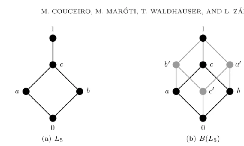
(a)L5 (b)B(L5)

Figure 1. A distributive lattice and its Boolean algebra

and sufficient conditions for the existence of an interpolating lattice polynomial function. Goodstein’s theorem [15] provides a solution in the special case when the domain ofgis the hypercubeD={0,1}ⁿ, where 0 and 1 are the least and greatest elements of the bounded distributive lattice L: a function g:{0,1}ⁿ → L can be interpolated by a polynomial functionp: Lⁿ→Lif and only ifgis monotone, and in this case p is unique. This result was generalized in [11] by allowing L to be an arbitrary (possibly unbounded) distributive lattice and by considering functions g:D→L, whereD={a1, b₁} × · · · × {an, b_n}witha_i, b_i∈Landa_i< b_i, for each i∈[n].

To describe the general solution of the Polynomial Interpolation Problem, which was given in [5], we need to recall that by the Birkhoff-Priestley representation theorem [12] we can embed any distributive lattice L into a Boolean algebra B, which can be assumed to be a subalgebra of the power setP(Ω) of a set Ω. For the sake of canonicity, we assume thatLgeneratesB, so thatB is uniquely determined up to isomorphism. The complement of an elementa∈B is denoted by a⁰. (See Figure 1 for an example.)

Given a functiong:D→L, we define the following two elements inB for each I⊆[n]:

c⁻_I := _

a∈D

g(a)∧^

i /∈I

a⁰_i

and c⁺_I := ^

a∈D

g(a)∨_

i∈I

a⁰_i .

Observe thatI⊆J impliesc⁻_I ≤c⁻_J andc⁺_I ≤c⁺_J. Letp⁻andp⁺be the polynomial functions overB given by these two systems of coefficients:

p⁻(y) := _

I⊆[n]

c⁻_I ∧^

i∈I

yi

and p⁺(y) := _

I⊆[n]

c⁺_I ∧^

i∈I

yi

.

As it turns out [5],p⁻andp⁺are the least and greatest polynomial functions over B whose restriction to D coincides with g (whenever such a polynomial function exists). This yields the following explicit description of all possible interpolating polynomial functions over the Boolean algebraB.

Theorem 1([5]). Let Lbe a distributive lattice, and let B be the Boolean algebra generated by L. Let g:D →L be a function defined on a finite set D ⊆Lⁿ, and let p:Bⁿ → B be a polynomial function over B given by (2). Then the following conditions are equivalent:

(5)

(i) pinterpolatesg, i.e.,p|D=g;

(ii) c⁻_I ≤cI ≤c⁺_I for all I⊆[n];

(iii) p⁻ ≤p≤p⁺.

From Theorem 1 it follows that a necessary and sufficient condition for the existence of a polynomial function p: Bⁿ → B such that p|D = g is c⁻_I ≤ c⁺_I, for every I ⊆ [n]. Moreover, if for every I ⊆ [n], there is cI ∈ L such that c⁻_I ≤cI ≤c⁺_I, then and only then there is a polynomial function p:Lⁿ →Lsuch that p|D=g. For the special type of interpolation problem considered in [11], the condition for the existence of a solution was given by simple lattice inequalities, without referring to the Boolean algebra generated by the lattice. In the case when Lis a finite chain such a condition was given in [23], where, rather than polynomial functions, the interpolating functions where assumed to be Sugeno integrals, i.e., idempotent polynomial functions (see [18, 19]). One can also obtain the solution of the Polynomial Interpolation Problem over L in this case from Theorem 1 by describing explicitly the Boolean algebra generated by a finite chain. This yields the following result, which basically reformulates Theorem 3 in [23] in the language of lattice theory [5].

Theorem 2([23]). LetLbe a finite chain, and letg:D→Lbe a function defined on a subset D ⊆Lⁿ. Then there is a polynomial function p: Lⁿ → L such that p|D=g if and only if

(3) ∀a,b∈D: g(a)< g(b) =⇒ ∃i∈[n] :ai≤g(a)< g(b)≤bi.

In contrast to the above mentioned special cases, in general it is not possible to avoid the use of the Boolean algebra generated by L, as it is illustrated by the following example.

Example 3 ([5]). Let L5 be the five-element lattice shown in Figure 1a, and let B(L5) be the Boolean algebra generated by L5 (see Figure 1b). Let D ={a,b}, wherea= (1, c),b= (c, a) and considerg:D→L5 defined by

(4) g(a) = 1 and g(b) =a.

As coefficientsc⁻_I andc⁺_I we obtain

c⁻_∅ = 0, c⁻_{1}=c⁰, c⁻_{2} = 0, c⁻_{1,2}= 1, c⁺_∅ =a, c⁺_{1}=b⁰, c⁺_{2}= 1, c⁺_{1,2}= 1.

We see thatc⁻_I ≤c⁺_I holds for eachI⊆[2], hence this interpolation problem has a solution overB(L5) (in fact, it has 32 solutions), by Theorem 1. On the other hand, no element ofL5 lies betweenc⁻_{1} andc⁺_{1}, hence there is no solution over L5.

3. Generalized lattice interpolation

As mentioned in the introduction, the motivation for considering the interpolation problem is rooted in the qualitative approach to preference modeling, where preference relations over a setX₁× · · · ×X_n of alternatives described byn attributes are represented by overall utility functions U:X₁× · · · ×X_n →Lvalued in an ordered setL, by the rule:

xy if and only if U(x)≤U(y).

(6)

Preferences on the attributes Xi are in turn modeled by local utility functions ϕi: Xi →L, which are then aggregated through a lattice polynomial p: Lⁿ → L thus giving rise to refined models

(5) U(x) =p ϕ1(x1), . . . , ϕn(xn) , which we referred to aspseudo-polynomial functions.

The interest of considering the interpolation problem in this setting becomes apparent when dealing with preference relations that are partially defined. This situation of incomplete information pertains to preference learning, where the set of interpolating pseudo-polynomial functions constitutes its version space. This mo- tivates the following extension of the interpolation problem (stated as Problem 5.1 in [11]):

Pseudo-polynomial Interpolation Problem. LetX1, . . . , Xnbe finite sets and L a finite distributive lattice. Given C ⊆ X1× · · · ×Xn and a partial function f:C→L, find all pseudo-polynomial functionsU:X1× · · · ×Xn →L such that U|C=f.

As mentioned in Section 1, uncertainty can be modeled by special kinds of pseudo-polynomials, where X₁ = · · · = X_n = X and ϕ₁ = · · · = ϕ_n = ϕ. The resulting global utilty functions U: Xⁿ → L are so-called quasi-polynomial functions:

(6) U(x) =p ϕ(x₁), . . . , ϕ(x_n) .

The corresponding interpolation problem can be formulated as follows:

Quasi-polynomial Interpolation Problem. LetX be a finite set andLa finite distributive lattice. Given C ⊆ Xⁿ and a partial function f: C → L, find all quai-polynomial functionsU:Xⁿ→Lsuch thatU|C=f.

We present the solution of the Pseudo-polynomial Interpolation Problem in two steps. First, in Subsection 3.1 we show how to find the appropriate polynomials pprovided that the local utility functions ϕ₁, . . . , ϕ_n are given. Then, in Subsec- tion 3.2 we give an algorithm to construct all possible local utility functions that could appear in an interpolation. To simplify the formalism, in Subsection 3.2 we consider the special case of quasi-polynomials, but our method can be easily adapted to the more general problem of pseudo-polynomial interpolation, see Remark 8.

3.1. Interpolation with known local utility functions. Assume that the local utility functionsϕi:Xi→Lare given; our goal is to find all polynomial functionsp overLsuch that the pseuo-polynomial functionU given by (5) interpolatesf. Let us consider an arbitrary polynomial functionpoverBin its disjunctive normal form (2). The corresponding pseudo-polynomial functionU =p(ϕ1, . . . , ϕn) interpolates f if and only if p(ϕ1(a1), . . . , ϕn(an)) = f(a1, . . . , an) for all a ∈ C, i.e., if p interpolates the functiong:D→Ldefined on the set

D={(ϕ1(a1), . . . , ϕn(an)) :a∈C}

by

g(ϕ₁(a₁), . . . , ϕ_n(a_n)) =f(a₁, . . . , a_n).

(7)

Using the construction of Section 2 for this interpolation problem, we can define coefficientsc⁻_I,ϕ

1,...,ϕ_n andc⁺_I,ϕ

1,...,ϕ_n for everyI⊆[n] as follows:

c⁻_I,ϕ

1,...,ϕ_n:= _

a∈C

f(a)∧^

i /∈I

ϕi(ai)⁰

and c⁺_I,ϕ

1,...,ϕ_n := ^

a∈C

f(a)∨_

i∈I

ϕi(ai)⁰ .

Denoting the corresponding polynomial functions byp⁻_ϕ

1,...,ϕ_n andp⁺_ϕ

1,...,ϕ_n, Theo- rem 1 yields the following solution for the Pseudo-polynomial Interpolation Problem with known local utility functions.

Theorem 4. LetX₁, . . . , X_n be finite sets, letLbe a finite distributive lattice, and let f: C → L be a function defined on a set C ⊆ X₁× · · · ×X_n. For any maps ϕ_i: X_i→L(i∈[n])and any polynomial functionp:Bⁿ→B overB given by (2), the following conditions are equivalent:

(i) U =p(ϕ₁, . . . , ϕ_n)interpolates f, i.e.,U|_C=f; (ii) c⁻_I,ϕ

1,...,ϕn ≤c_I ≤c⁺_I,ϕ

1,...,ϕn for allI⊆[n];

(iii) p⁻_ϕ

1,...,ϕ_n≤p≤p⁺_ϕ

1,...,ϕ_n.

Remark 5. Note that if there exist tuples a,b ∈ C such that f(a) 6= f(b) but (ϕ1(a1), . . . , ϕn(an)) = (ϕ1(b1), . . . , ϕn(bn)), then it is clearly impossible to find an interpolating pseudo-polynomial function (or any kind of function at all).

We invite the reader to verify that this situation cannot occur if condition (ii) of Theorem 4 is satisfied.

3.2. Interpolation with unknown local utility functions. Now let us consider interpolation by quasi-polynomial functions

U(x) =p(ϕ(x1), . . . , ϕ(xn)),

where the local utility function ϕ: X → L is not known. Our aim is to find all possible maps ϕ for which an interpolating polynomial exists. Specializing the results of the previous subsection to the case ϕ₁ = · · · = ϕ_n = ϕ, we see that the necessery and sufficient condition for the existence of a solution overB is that c⁻_I,ϕ≤c⁺_I,ϕfor allI⊆[n], where

c⁻_I,ϕ:= _

a∈C

f(a)∧^

i /∈I

ϕ(a_i)⁰

and c⁺_I,ϕ:= ^

a∈C

f(a)∨_

i∈I

ϕ(a_i)⁰ . Equivalently, we must have

(7) ∀a,b∈C ∀I⊆[n] : f(a)∧^

i /∈I

ϕ(ai)⁰ ≤f(b)∨_

i∈I

ϕ(bi)⁰.

Thus, we have a system of inequalities for the unknown values ϕ(a) (a∈X).

To find all solutions of this system of inequalities, we make use of the fact thatB can be embedded into the power set of a set Ω. We will encode a map ϕ: X → B by a system of sets Sω ⊆ X(ω∈Ω), where Sω = {a∈X:ω∈ϕ(a)}. It is straightforward to verify that the inequalities (7) translate to the following condition for the setsSω:

(8) ∀ω∈f(a)\f(b) ∀I⊆[n] : {b_i:i∈I} ⊆S_ω =⇒ {a_i:i /∈I} ∩S_ω6=∅.

(Heref(a)\f(b) is the difference of the sets f(a), f(b)⊆Ω.)

Observe that for given ω ∈ Ω and a,b ∈ C, it is sufficient to consider the set I ={i∈[n] : b_i∈S_ω} in (8) instead of all subsets of [n], since this gives the strongest condition. Hence we may constructS_ωby starting with the empty set, and

(8)

Algorithm 1Constructing all possible setsS_ω

1: Sω:=∅

2: computeE by (9)

3: repeat

4: add a covering set of H= (X,E) toSω 5: recomputeE by (9)

6: untilE =∅ or∅ ∈ E

7: if E=∅ then

8: return S_ω

9: else

10: return fail

11: end if

adding an element of{ai:i /∈I}if necessary, for alla,b∈Cwithω∈f(a)\f(b) andI={i∈[n] : bi∈Sω}. However, note that we must not add too many elements toSω, since if {bi:i∈[n]} ⊆Sω, then (8) yields the contradiction∅ ∩Sω6=∅.

At any stage of this process, let us collect all the sets{ai: i /∈I} of which we must add an element toSω:

(9) E:=n

{ai:i /∈I} : a,b∈C, ω∈f(a)\f(b),

I={i∈[n] : bi∈Sω},{ai:i /∈I} ∩Sω=∅o . This way we obtain a hypergraph H = (X,E), and condition (8) requires that a vertex cover (i.e., a set of vertices intersecting every hyperedge) of Hbe included inSω. This yields Algorithm 1 for constructingSω.

The algorithm terminates when eitherE =∅, which means that (8) is satisfied, hence we do not need to add any more elements toSω, or∅ ∈ E, which means that the above mentioned contradiction ∅ ∩Sω 6= ∅ occurs, and it cannot be resolved by adding more elements to S_ω. In order to make sure that we find all possible solutions, we must try every covering set of Hin line 4 of the algorithm in every iteration. If we would like to find just one solution (if there is one at all), then it is sufficient to add a minimal covering set ofH, but still we must tryevery minimal covering set in every iteration, leading to an exponential running time.

Remark 6. The example of Section 4 shows that this cannot be avoided, since it is possible that certain covering sets may lead to a contradiction, while other covering sets give a solution. Also, in Section 5 we prove that even deciding the existence of an interpolating quasi-polynomial function is an NP-complete problem, hence an effective algorithm cannot be expected unless P = NP.

To determine the whole version space, i.e., the set of all interpolating quasi- polynomial functions, one needs to compute all possible systems of setsSω(ω∈Ω), and then one can define the corresponding local utility functions ϕ:X → B by ϕ(a) ={ω∈Ω :a∈S_ω}. After computing all such mapsϕ, one can select those for whichϕ(a)∈Lholds for alla∈X. Then using the construction of Subsection 3.1 one can determine the corresponding polynomial functions p for each ϕ. Recall that the coefficientsc⁻_I,ϕ, c⁺_I,ϕbelong toB, but we need only the elements ofLthat lie betweenc⁻_I,ϕandc⁺_I,ϕ.

(9)

Example 7. Note that the current setting is strictly more general than that of the previous section. To illustrate this, let X = {0, a,1} = L and C = {(0,1),(1,0),(a, a),(1,1)}. (The ordering on L is 0 < a < 1, i.e., L is a three- element chain. ThenB can be chosen as {0, a, a⁰,1} with 0< a, a⁰ <1.) Consider f:C→Lgiven by

f(a, a) = 0,

f(0,1) =f(1,0) =a, f(1,1) = 1.

Using Theorem 1, we can verify that there is no polynomial function that would interpolate f on C (even if considered over the Boolean lattice B extending L).

However, takingϕ:X →Lgiven byϕ(0) =ϕ(a) = 0 andϕ(1) = 1, we get c⁻_∅,ϕ=c⁺_∅,ϕ= 0,

c⁻_{1},ϕ=c⁺_{1},ϕ=c⁻_{2},ϕ =c⁺_{2},ϕ=a, c⁻_{1,2},ϕ=c⁺_{1,2},ϕ= 1.

Hence,p=p⁻_ϕ =p⁺_ϕ = (a∧x1)∨(a∧x2)∨(1∧x1∧x2), and it is not difficult to verify thatU =p◦ϕindeed interpolatesf.

Remark 8. Let U:X1× · · · ×Xn → L be a pseudo-polynomial function of the form (5). Assume (without loss of generality) that the setsX₁, . . . , X_nare pairwise disjoint, and let X =X₁∪ · · · ∪X_n and ϕ= ϕ₁∪ · · · ∪ϕ_n. Consider the quasi- polynomial functionUe:Xⁿ →L defined byUe(x) =p ϕ(x₁), . . . , ϕ(x_n)

. Observe that X1 × · · · ×Xn ⊆ Xⁿ and the restriction of Ue to X1 × · · · ×Xn coincides withU. Thus, every pseudo-polynomial function can be viewed as a restriction of a quasi-polynomial function. Conversely, ifp ϕ(x1), . . . , ϕ(xn)

is a quasi-polynomial function over X, then its restriction to X₁ × · · · ×X_n is a pseudo-polynomial function corresponding to the local utility functionsϕ_i=ϕ|Xi(i= 1, . . . , n). This observation allows us to use Algorithm 1 almost verbatim to solve the Pseudo- polynomial Interpolation Problem.

4. A case study

We illustrate the construction of the version space outlined in the previous section on the example mentioned in Section 1. Our setup is the following:

• L ={0, a,1}, where 0 means “quit job”, ameans “continue job but look for alternatives” and 1 means “continue job”. We take the natural ordering 0< a <1 onL.

• X ={E,P,M,D}, where E means “excellent”, P means “physically down”, M means “mentally down” and D means “depressed”. We do not need an order structure onX, however, it seems natural to considerEandDas the best and worst cases, andPandMlie between them: D<P,M<E.

• C={(P,E,D,P),(E,D,P,P),(D,E,M,M),(P,M,E,D),(M,M,E,P)}, andf:C→ Lis given by

f(P,E,D,P) = 0, f(P,M,E,D) = 1, f(E,D,P,P) =a, f(M,M,E,P) = 1, f(D,E,M,M) =a.

(10)

The lattice L can be embedded into the power set of a two-element set Ω = {ω1, ω2}, hence we haveB=P(Ω), and we regard the elements of Las subsets of Ω:

0 =∅, a={ω₁}, 1 ={ω₁, ω₂}.

Note that B = {0, a, a⁰,1}, wherea⁰ = {ω₂}. One can interpretω₁ as “continue job” and ω₂ as “do not look for alternatives”. Thena⁰ would mean “quit job but do not look for alternatives”, which is naturally excluded from the set of possible options.

Let us compute (some of) the possible sets Sω₁ that satisfy (8). Starting with Sω₁ =∅we haveE =

{E,P,M,D},{E,M,D},{E,P,D},{E,P,M} by (9). The hypergraph H = (X,E) has 4 minimal covering sets, namely {E},{P,M},{P,D},{M,D}.

Any subset ofX containing one of these sets is a covering set; there are altogether 12 covering sets, and we should examine each one of them in order to find all solutions. This is rather tedious, hence we give the details only for the minimal covering sets.

Setting Sω1 ={E}, we obtainE =

{M,D} , hence we must add eitherMor Dto S_ω₁. In the former case we get E =∅, which yields the solution S_ω₁ ={E,M}. In the latter case we haveS_ω₁ ={E,D}and E=

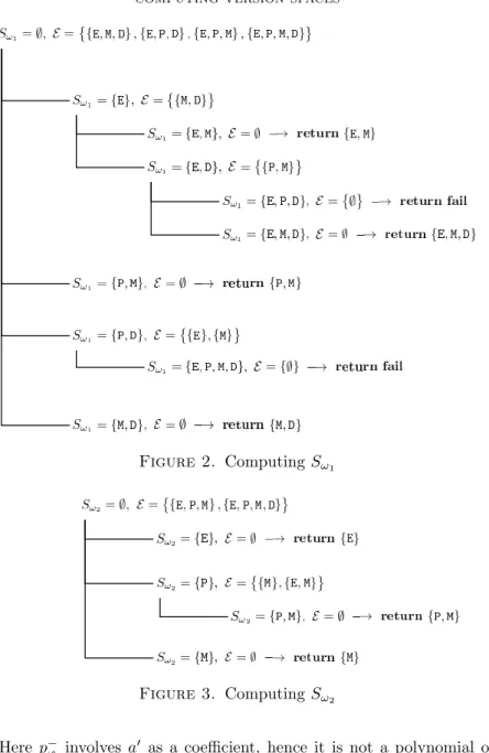
{P,M} , hence one ofPandMmust be added to S_ω₁. The case S_ω₁ ={E,P,D} givesE ={∅}, and the corresponding hypergraph has no covering sets. The case S_ω₁ ={E,M,D} givesE =∅, and this means that there are no edges that need to be covered, i.e.,S_ω₁ ={E,M,D}satisfies (8). The rest of the computation is shown on Figure 2. Note that if we had started withSω₁={P,D}instead ofSω₁ ={E}at the beginning, then we would have gotten no solutions. This illustrates that one must search the whole tree of possibilities in order to guarantee that a solution will be found if there is one.

Figure 3 shows the computations for Sω₂, again only working with minimal covering sets. Taking into account non-minimal covering sets as well, one obtains all possible setsSω₁ and Sω₂:

Sω₁: {E,M}, {P,M}, {M,D}, {E,P,M}, {E,M,D}; Sω₂: {E}, {M}, {P,M}, {M,D}, {E,P,M}, {P,M,D}.

There are 30 possibilties for the systems of setsSω(ω∈Ω), hence there are 30 maps ϕ: X →B for which an interpolating polynomial exists over B. However, if there is an elementu∈Sω₂\Sω₁, thenϕ(u) =a⁰ ∈/ L. Therefore, it sufficies to consider the cases whereSω₂ ⊆Sω₁, giving 13 local utility functionsϕ: X→L.

If we consider the partial orderingD<P,M<EonX and we look only for order- preserving maps ϕ, then we have only 3 possibilities. We give the corresponding polynomial functionsp⁻_ϕ andp⁺_ϕ only for these cases (for easier readability we omit the∧signs and write meets simply as juxtapositions):

• Sω₁={E,P,M}, Sω₂ ={E,P,M}: In this case we have ϕ(E) = 1, ϕ(P) = 1, ϕ(M) = 1, ϕ(D) = 0;

p⁻_ϕ =y₁y₂y₃∨ay₁y₃y₄∨ay₂y₃y₄, p⁺_ϕ =ay₃∨y₁y₂y₃.

• S_ω₁={E,M}, S_ω₂ ={E}: In this case we have

ϕ(E) = 1, ϕ(P) = 0, ϕ(M) =a, ϕ(D) = 0;

p⁻_ϕ =ay₁∨a⁰y₃∨y₁y₃∨y₂y₃, p⁺_ϕ =ay₁∨y₃∨y₄∨y₁y₂.

(11)

Figure 2. ComputingSω₁

Figure 3. ComputingS_ω₂

Here p⁻_ϕ involves a⁰ as a coefficient, hence it is not a polynomial over L.

The least polynomialpoverLsatisfyingp⁻_ϕ ≤pis obtained by replacinga⁰ by 1:

p=ay₁∨1y₃∨y₁y₃∨y₂y₃=ay₁∨y₃.

Probably this is the simplest polynomial over Lthat lies between p⁻_ϕ and p⁺_ϕ; the corresponding quasi-polynomial U(x) =aϕ(x₁)∨ϕ(x₃) depends only on x₁ and x₃, which shows that it suffices to evaluate the person’s well-being in winter and summer in order to choose the action to take.

• S_ω₁={E,P,M}, S_ω₂ ={E}: In this case we have ϕ(E) = 1, ϕ(P) =a, ϕ(M) =a, ϕ(D) = 0;

p⁻_ϕ =a⁰y₃∨y₁y₂y₃∨y₁y₃y₄∨y₂y₃y₄, p⁺_ϕ =y₃∨a⁰y₄∨a⁰y₁y₂.

(12)

Againa⁰ appears in the polynomials; we need to replce it by 1 in p⁻_ϕ and by 0 in p⁺_ϕ to all find polynomials poverL such thatp⁻_ϕ ≤p≤p⁺_ϕ. After simplification, we get the polynomial y3 in both cases. This means that for this local utility function the interpolating quasi-polynomial is unique:

U(x) = ϕ(x3); revealing the fact that x3 (i.e., the person’s well-being in summer) alone can determine the recommended action to take.

5. Complexity of quasi-polynomial interpolation

In Section 3 we gave an algorithm that constructs all quasi-polynomial functions interpolating a given partial functionf:C→L (C⊆Xⁿ). We noticed that even if one looks for only one interpolating quasi-polynomial, the algorithm still involves finding minimal covering sets in hypergraphs, which is an NP-complete problem [14]. In this section we prove that this difficulty is not avoidable, as already for n = 4, it is an NP-complete problem to decide whether an interpolating quasi- polynomial exists. However, as we shall see, for n≤3 this problem can be solved in polynomial time. For background on complexity theory we refer the reader to [14].

First let us observe that it is sufficient to consider the case whereL is the two- element lattice. Indeed, if L is any finite distributive lattice, then, as before, we embedL into a power setP(Ω) of a finite set Ω, and consider the elementsω∈Ω separately, as we did in (8). In this way we can translate the Quasi-polynomial Interpolation Problem to |Ω| many problems with two-element lattices P({ω}).

Therefore, in the sequel we will always assume thatL={0,1}.

We will examine the complexity of our interpolation problem with the help of certain constraint satisfaction problems that are related to upsets in the Boolean latticeLⁿ={0,1}ⁿ. We say that a subsetα⊆Lⁿis anupset(order filter) ifa1∈α anda1≤a2 (in the componentwise ordering) implya2∈αfor alla1,a2∈Lⁿ. We will denote the complement ofαbyβ, i.e.,β=Lⁿ\α. Observe thatβis adownset (order ideal): b1 ∈β and b1 ≥b2 imply b2 ∈ β for all b1,b2 ∈Lⁿ. For every upsetα⊆Lⁿ we define a problemP(α) as follows.

Problem P(α). Given a finite setV of variables and sets ofn-tuplesA, B ⊆Vⁿ, find an assignmentψ: V →Lsuch that ψ(a)∈α for alla ∈Aand ψ(b)∈β = Lⁿ\αfor allb∈B.

Note thatP(α) is a Boolean constraint satisfaction problem, hence, by Schaefer’s dichotomy theorem for Boolean CSP, it is either in P or NP-complete [24].

Lemma 9. Let L = {0,1} be the two-element lattice, let X be a finite set and f:C →L (C⊆Xⁿ). There exists a quasi-polynomial function interpolating f if and only ifP(α)has a solution for some upsetα⊆Lⁿ with V =X and

A={a∈C: f(a) = 1}, B={b∈C:f(b) = 0}.

Proof. As we have seen in Section 3, an interpolating quasi-polynomial exists if and only if there is a map ϕ:X → L satisfying (7). If f(a) = 0 or f(b) = 1, then the inequality of (7) clearly holds for all I ⊆ [n]. For f(a) = 1 and f(b) = 0, the inequality holds for all I ⊆ [n] if and only if there is an index i ∈ [n] such thatϕ(a_i) = 1 andϕ(b_i) = 0, i.e.,ϕ(a)ϕ(b) in the componentwise ordering of n-tuples overL={0,1}. Thus, (7) is equivalent to the following condition:

(10) ∀a,b∈C: (f(a) = 1 andf(b) = 0) =⇒ ϕ(a)ϕ(b).

(13)

(Note that the implication in (10) can be reformulated as ϕ(a) ≤ ϕ(b) =⇒ f(a)≤f(b). This gives an alternative way of proving that (10) is equivalent to the existence of a polynomialpsuch thatf(c) =p(ϕ(c)) for allc∈C, since lattice polynomial functions coincide with nondecreasing functions over the two-element lattice.)

Assume thatϕsatisfies (10), and letαbe the least upset containingϕ(a) for all a∈A:

α:={y∈Lⁿ:y≥ϕ(a) for somea∈A}.

Obviously, we haveϕ(a)∈αfor alla∈A, and (10) implies thatϕ(b)∈/αfor all b∈B. Thus,ϕis a solution of the problemP(α) withXbeing the set of variables.

Conversely, ifα⊆Lⁿ is an arbitrary upset andϕis a solution ofP(α), then it

is immediate thatϕsatisfies (10).

According to Lemma 9, we can split the Quasi-polynomial Interpolation Problem into finitely many subproblemsP(α) with αrunning through the set of upsets of Lⁿ. If each of these subproblems can be solved in polynomial time, then the whole problem is in P. As the next theorem shows, this is the case forn≤3.

Theorem 10. If n≤3, then the problem of deciding the existence of an interpolating quasi-polynomial function belongs to the complexity classP.

Proof. Clearly, it suffices to prove the theorem forn= 3. By Lemma 9, we only need to show thatP(α) is in P for every upsetα⊆L³. Up to permutations of variables, we have the 8 cases listed below. For each upset αwe give a polymorphism hof the constraint language {α, β} that shows that P(α) belongs to P by Schaefer’s dichotomy theorem. (For better readability we write elements ofL³ as words.)

α={111} h=x∧y

α={101,111} h=x∧y

α={101,110,111} h= (x∧y)∨(x∧z)∨(y∧z) α={100,101,110,111} h=x∧y

α={011,101,110,111} h= (x∧y)∨(x∧z)∨(y∧z) α={011,100,101,110,111} h= (x∧y)∨(x∧z)∨(y∧z) α={010,011,100,101,110,111} h=x∨y

α={001,010,011,100,101,110,111} h=x∨y

Forn≥4 one can find upsetsα⊆Lⁿsuch thatP(α) is NP-complete. This does not yield immediately NP-completeness of the interpolation problem, since there might be “easy” solutions corresponding to some other upsets. Nevertheless, in the next theorem we prove that the Quasi-polynomial Interpolation Problem is indeed NP-complete forn≥4.

Theorem 11. If n≥4, then the problem of deciding the existence of an interpolating quasi-polynomial function isNP-complete.

Proof. Clearly, it suffices to prove the theorem for n = 4. Let α ⊆ {0,1}⁴ be the upset consisting of tuples of Hamming weight at least 3, that is, α :=

{0111,1011,1101,1110,1111}. In this case the constraint language {α, β} admits only projections as polymorphisms, thus P(α) is NP-complete, by Schaefer’s dichotomy theorem.

(14)

For every instance of P(α) we construct an instance of the quasi-polynomial interpolation problem with L = {0,1} and n = 4 such that the solutions ψ of the former are in a one-to-one correspondence with the local utility functions ϕ that solve the latter. So assume that V and A, B ⊆ V⁴ are given, as in P(α).

Let X = V ∪ {0,˙ 1}, C =A∪B∪ {0,˙ 1}⁴ (where ˙∪ denotes disjoint union) and f:C→L⁴ such that

∀a∈A∪α:f(a) = 1 and ∀b∈B∪β:f(b) = 0.

(Note that 0 and 1 belong to bothX andL, hence they play the role of “variables”

as well as the role of “values”.) We claim that a map ϕ:X → L satisfies (10), which, as we have seen in Lemma 9, is equivalent to (7), if and only if ϕ(0) = 0 andϕ(1) = 1, and the restrictionψ:=ϕ|V ofϕtoV is a solution ofP(α).

First suppose thatϕsatisfies (10). This immediately implies thatϕ(a)ϕ(b) for alla∈αand b∈β, and it easy to see that this holds if and only ifϕ(0) = 0 andϕ(1) = 1. Now applying (10) witha∈A,b∈β, we getϕ(a)ϕ(b) =b; in particular, ϕ(a)6=b. Since this holds for allb∈ β, we have thatϕ(a)∈/ β, i.e., ϕ(a)∈α. A similar argument shows thatϕ(b)∈β for allb∈B, and this proves thatψ=ϕ|V is indeed a solution toP(α).

Next assume that ψ is a solution of P(α), and let ϕ: X →L coincide with ψ onV, and let ϕ(0) = 0,ϕ(1) = 1. Then we have ϕ(a)∈α for all a∈A∪α(if a ∈A then by the costraints of P(α), ifa ∈αthen by the fact that ϕ(a) =a), and similarly,ϕ(b)∈β for all b∈ B∪β. Therefore, if f(a) = 1 and f(b) = 0, thenϕ(a)∈αandϕ(b)∈β, and this implies thatϕ(a)ϕ(b), hence (10) holds.

This proves that the Quasi-polynomial Interpolation Problem for n = 4 and L={0,1}can be reduced in polynomial time toP(α), showing that the former is

also NP-complete.

Summarizing Theorems 10 and 11, we obtain the following dichotomy result.

Corollary 12. If n≤3 then the problem of deciding the existence of an interpolating quasi-polynomial function is in P, whereas forn≥4it isNP-complete.

6. Concluding remarks and future work

In this paper we considered the problem of interpolating empirical data given as couples consisting of a tuple specified by several attributes, together with its evaluation in a distributive lattice. The interpolating objects are lattice-valued functions, called quasi- and pseudo-polynomial functions, that can be factorized into a composition of a lattice polynomial function with possibly different local utility functions that evaluate each attribute in a distributive lattice. We presented necessary and sufficient conditions for the existence of quasi- and pseudo-polynomial functions interpolating a given finite set of examples. In doing so, we actually presented explicit descriptions of such solutions when they exist. Looking into complexity issues in computing them, we established a dichotomy result stating that, up to 3 attributes, the existence of an interpolationg quasi-polynomial function can be decided in polynomial time, whereas this problem for sets of examples over more than 3 attributes becomes NP-complete. The analogous complexity question for pseudo-polynomial functions remains open.

Now our framework was motivated by problems typically arising in the qualitative approach to multicriteria decision making. The basic aggregation functions

(15)

considered, namely, lattice polynomial functions (that include Sugeno integrals), have neat representations, e.g., by disjunctive normal forms, and played a key role in the constructions provided. Other noteworthy aggregation functions in decision making, such as Lov´asz extensions (that include Choquet integrals), also share similar representation features. The natural step is to make use them when considering analogous interpolation problems for these aggregation models.

Furthermore, simplified notions of Sugeno and Choquet integrals (parametri- zed versions arising from the notions of k-maxitivity and k-additivity; see [16]

for a general reference) have been proposed in the literature and could provide alternatives to avoid intractable complexity classes when dealing with interpolation problems.

These constitute few topics of our current interest, and that will be tackled in forthcoming research work.

References

[1] D. Bouyssou, T. Marchant, M. Pirlot. A conjoint measurement approach to the discrete Sugeno integral, pp. 85–109, inThe Mathematics of Preference, Choice and Order. Essays in Honor of Peter C. Fishburn, Brams, S., Gehrlein, W. V., Roberts, F. S. (Eds.), 2009.

[2] K. Cao-Van, B. De Baets, S. Lievens. A probabilistic framework for the design of instance- based supervised ranking algorithms in an ordinal setting,Annals Operations Research163 (2008) 115–142.

[3] A. Cornu´ejols, L. Miclet.Apprentissage artificiel - Concepts et algorithmes, Eyrolles, 2010 [4] M. Couceiro, D. Dubois, H. Prade, T. Waldhauser. Decision-making with Sugeno integrals.

Bridging the gap between multicriteria evaluation and decision under uncertainty. To appear inOrder, 15 pages.

[5] M. Couceiro, D. Dubois, H. Prade, A. Rico, T. Waldhauser. General interpolation by polynomial functions of distributive lattices. Information Processing and Management of Uncertainty in Knowledge-Based Systems,Communications in Computer and Information Science, vol.

299, Springer-Verlag, 347-355, 2012.

[6] M. Couceiro, J.-L. Marichal. Characterizations of discrete Sugeno integrals as polynomial functions over distributive lattices,Fuzzy Sets and Systems 161:5 (2010) 694–707.

[7] M. Couceiro, J.-L. Marichal. Axiomatizations of quasi-polynomial functions on bounded chains,Aequationes Mathematicae78:1 (2009) 195–213.

[8] M. Couceiro, J.-L. Marichal. Quasi-polynomial functions over bounded distributive lattices, Aequationes Mathematicae80(2010) 319–334.

[9] M. Couceiro, T. Waldhauser. Axiomatizations and factorizations of Sugeno utility functions, Internat. J. Uncertain. Fuzziness Knowledge-Based Systems 19:4 (2011) 635–658.

[10] M. Couceiro, T. Waldhauser. Pseudo-polynomial functions over finite distributive lattices, Fuzzy Sets and Systems 239(2014) 21–34.

[11] M. Couceiro, T. Waldhauser. Interpolation by polynomial functions of distributive lattices:

a generalization of a theorem of R. L. Goodstein,Algebra Universalis69:3 (2013) 287–299.

[12] B. A. Davey, H. Priestley.Introduction to Lattices and Order, Cambridge University Press, New York, 2002.

[13] J. F¨urnkranz, E. H¨ullermeier (eds.).Preference learning, Springer, Berlin, 2011.

[14] M. R. Garey, D. S. Johnson, Computers and intractability. A guide to the theory of NP- completeness, A Series of Books in the Mathematical Sciences, W. H. Freeman and Co., San Francisco, CA, 1979.

[15] R. L. Goodstein. The Solution of Equations in a Lattice,Proc. Roy. Soc. EdinburghSection A67(1965/1967) 231–242.

[16] M. Grabisch, J.-L. Marichal, R. Mesiar, E. Pap. Aggregation Functions, Encyclopedia of Mathematics and Its Applications127, Cambridge University Press, Cambridge, 2009.

[17] S. Greco, B. Matarazzo, R. S lowi´nski. Axiomatic characterization of a general utility function and its particular cases in terms of conjoint measurement and rough-set decision rules, European Journal of Operational Research158(2004) 271–292.

(16)

[18] J.-L. Marichal. On Sugeno integral as an aggregation function,Fuzzy Sets and Systems114 (2000) 347–365.

[19] J.-L. Marichal. Weighted lattice polynomials,Discrete Mathematics309:4 (2009) 814–820.

[20] T. Mitchell,Machine Learning, McGraw Hill, 1997

[21] H. Prade, A. Rico, M. Serrurier. Elicitation of Sugeno Integrals: A version space learning perspective. Proc. 18th Inter. Symp. on Methodologies for Intelligent Systems (ISMIS’09), (J. Rauch, Z. W. Ras, P. Berka, T. Elomaa, eds.), Prague, Sept. 14-17, Springer, LNCS 5722, 392–401.

[22] H. Prade, A. Rico, M. Serrurier, E. Raufaste. Eliciting Sugeno integrals: Methodology and a case study, 2009, in Proc. European Conf. on Symbolic and Quantitative Approaches to Reasoning with Uncertainty, ECSQARU’09, LNCS, pages: 712–723.

[23] A. Rico, M. Grabisch, Ch. Labreuche, A. Chateauneuf. Preference modeling on totally ordered sets by the Sugeno integral,Discrete Applied Math.147:1 (2005) 113–124.

[24] T. J. Schaefer. The complexity of satisfiability problems. Conference Record of the Tenth Annual ACM Symposium on Theory of Computing (San Diego, Calif., 1978), pp. 216–226, ACM, New York, 1978.

[25] M. Sugeno.Theory of Fuzzy Integrals and its Applications. PhD thesis, Tokyo Institute of Technology, Tokyo, 1974.

[26] M. Sugeno. Fuzzy measures and fuzzy integrals – a survey. In: Gupta, M. M., Saridis, G. N., Gaines, B. R., (eds),Fuzzy automata and decision processes, pp. 89–102. North-Holland, New York, 1977.

[27] A.F. Tehrani, W. Cheng, E. H¨ullermeier. Preference Learning Using the Choquet Integral:

The Case of Multipartite Ranking,IEEE Transactions on Fuzzy Systems20:6 (2012) 1102–

1113.

(M. Couceiro)LORIA (CNRS - Inria Nancy Grand Est - Université de Lorraine) Equipe Orpailleur – Bat. B, Campus Scientifique B.P. 239, 54506 Vandœuvre-lès-Nancy, France and LAMSADE-CNRS, Université Paris-Dauphine, Place du Maréhal de Lattre de Tas- signy, 75116 Paris, France

E-mail address:miguel.couceiro@inria.fr

(M. Maróti)Bolyai Institute, University of Szeged, Aradi vértanúk tere 1, H-6720 Szeged, Hungary

E-mail address:mmaroti@math.u-szeged.hu

(T. Waldhauser)Bolyai Institute, University of Szeged, Aradi v´ertan´uk tere 1, H-6720 Szeged, Hungary

E-mail address:twaldha@math.u-szeged.hu

(L. Zádori) Bolyai Institute, University of Szeged, Aradi vértanúk tere 1, H-6720 Szeged, Hungary

E-mail address:zadori@math.u-szeged.hu