Polynomial inequalities and Green’s functions ∗
Vilmos Totik
†July 3, 2020
Abstract
The paper discusses some classical polynomial inequalities, their recent extensions to general sets, as well as the potential theory behind them. A unifying feature will be that in many cases the best constant is given in terms of the normal derivative of certain Green’s functions.
1 Classical inequalities
More than 100 years ago S. N. Bernstein proved in [7] his famous inequality1 for the derivatives of trigonometric polynomials
Tn(t) = a0
2 + (a1cost+b1sint) +· · ·+ (ancosnt+bnsinnt) of degree at mostn, namely for allθ
|Tn′(θ)| ≤nsup
t |Tn(t)|. (1)
This becomes an equality for example forTn(t) = sinnt andθ = 0. It will be convenient to rewrite it in the form
kTn′k ≤nkTnk,
where kTnk = supt|Tn(t)|is the supremum norm over the whole real line. In general, the supremum norm on a setE is defined as
kfkE= sup
t∈E|f(t)|. If
Pn(x) =anxn+an−1xn−1+· · ·+a0
∗AMS Classification 26D05, 42A05, Keywords: inequalities, trigonometric and algebraic polynomials, general sets, equilibrium density, Green’s functions, normal derivatives
†Supported by ERC Advanced Grant No. 267055
1Actually, the original [7] contained 2ninstead ofnin (1), see Section 6
is an algebraic polynomial of degree at mostn = 1,2, . . .2, then Pn(cost) is a trigonometric polynomial of degree at mostn, and for it (1) takes the form
|Pn′(x)| ≤ n
√1−x2kPnk[−1,1], x∈(−1,1), (2) which is again called “Bernstein’s inequality”. In it the right-hand side blows up asx→ ±1, and forxclose to±1 a better estimate is due to A. A. Markov [19] from 1890:
kPn′k[−1,1] ≤n2kPnk[−1,1]. (3)
2 Where are these polynomial inequalities used?
The polynomial inequalities from the previous section have various applications.
For example, one of the major tasks of approximation theory is the character- ization of the rate of approximation, say ofEn(f) = infTnkf −Tnk, where f is a 2π-periodic continuous function and the infimum is taken for all trigono- metric polynomials of degree at most n. From practical point of view one needs a computable quantity for the characterization, and such a quantity is smoothness, for example the Lipshitzαclass (Lipα) is defined by the property:
|f(x)−f(y)| ≤ M|x−y|α for all x, y with some M. A typical result is the following: for 0< α <1 the equivalence
f ∈Lipα ⇐⇒ En(f)≤ C
nα for someC
is true. The direction ⇒ can be proven by a direct construction like taking convolution with the Fej´er kernel, but in the direction⇐one needs Bernstein’s inequality. Indeed, suppose there are trigonometric polynomialsTn of degree at mostnsuch thatkf−Tnk ≤Cn−α. Then, by Bernstein’s inequality,
(T2k+1−T2k)′≤2k+1kT2k+1−T2kk ≤ 2k+1(kf−T2k+1k+kf−T2kk)
≤ 4C2k−α. (4)
Now for 2−n≤h≤2−n+1 we obtain, by the mean value theorem, with someξ in betweenxandx+h
|f(x)−f(x+h)| ≤ |f(x)−T2n(x)|+|f(x+h)−T2n(x+h)| + |T2n(x)−T2n(x+h)| ≤2C(2n)−α+h|T2′n(ξ)|, and, according to (4), here the last term is at most
h|T2′n(ξ)|=h
n−1X
k=−1
|T2′k+1(ξ)−T2′k(ξ)| ≤h
n−1X
k=−1
4C2k−α≤C1h2n−α≤C2hα,
2In what follows the degree ofPnis always assumed to be at mostn
(sinceT−1is constant). These show that|f(x+h)−f(x)| ≤C3hα, which is the Lipαproperty.
In fact, a large part of approximation theory deals with direct (smoothness
⇒ a given rate of approximation) and inverse (given rate of approximation
⇒smoothness) theorems, and the latter ones almost always involve a certain variant of the Bernstein or Markov inequalities.
In [14] Bernstein’s inequality played a decisive role in settling a conjecture in number theory on the uniform ditribution of the argument of so called ul- traflat polynomials (polynomialsPn(z) =P
kakzk with|ak|= 1, which satisfy
|Pn(z)| ≈ √n on the unit circle). It is also often used to estimate the val- ues of (trigonometric) polynomials at points in close proximity, see [6] or [14]
for such a use in number theory. Some other recent applications are related to heat diffusion [15], universality in random matrix theory [17], Hardy spaces [5], numerical analysis [24], Hilbert spaces [25], dynamical systems [16], partial differential equations [13], Fourier transforms [28], to name a few.
In the last 100 years many extensions and generalizations of the aforemen- tioned classical polynomial inequalities have been given. A particularly intensive period has been the last 20 years, during which very general forms have been found. To discuss them we need a few notions from potential theory. For a general reference to logarithmic potential theory see [27].
3 Equilibrium measures and Green’s functions
Let E ⊂ C be a compact subset of the plane. Think of E as a conductor, and put a unit charge on E, which can freely move in E. After a while the charge settles, it reaches an equilibrium. The mathematical formulation is the following (on the plane Coulomb’s law takes the form that the repelling force between charged particles is proportional with the reciprocal of the distance):
except for pathological cases, there is a unique probability measure µE onE, called the equilibrium measure ofE, that minimizes the energy integral
Z Z
log 1
|z−t|dµ(z)dµ(t) (5)
among all unit (Borel) measures supported on E. ThisµE certainly exists in all the cases we are considering in this paper.
WhenE⊂R, then we shall denote byωE(t) the density ofµEwith respect to Lebesgue measure wherever it exists. It certainly exists in the (one dimensional) interior ofE. For example,
ω[−1,1](t) = 1 π√
1−t2, t∈[−1,1],
is just the well known Chebyshev distribution. More generally, if TN is an algebraic polynomial of degreeN for which the complete inverse image
E=TN−1[−1,1] ={x TN(x)∈[−1,1]}
is part of the real line, then
ωE(t) = |TN′ (t)| πNp
1−TN(t)2, t∈E. (6)
In a similar fashion, ifEconsists of disjoint smooth Jordan curves and arcs with arc measure sE, then dµE = ωEdsE, and this ωE is called equilibrium density. For example, ifEis a circle of radiusr thenωE(z)≡1/2πronE. As another example, consider a lemniscate
σ={z |TN(z)|= 1},
whereTN is an algebraic polynomial of degreeN. Except for the points where σcrosses itself, we have
ωσ(z) =|TN′ (z)|/2πN.
For a further illustration, letE be a smooth (sayC2-smooth) Jordan curve (homeomorphic image of a circle) or arc (homeomorphic image of a segment), and Φ a conformal map from the exterior ofEonto the exterior of the unit circle C1(that maps the point infinity to itself). This Φ can be extended toEas a con- tinuously differentiable function (with the exception of the endpoints ofEwhen Eis a Jordan arc). Now ifEis a Jordan curve, then simplyωE(z) =|Φ′(z)|/2π.
IfEis a Jordan arc, then it has two sides, say positive and negative sides, and every pointz∈E different from the endpoints ofE is considered to belong to both sides, where they represent different pointsz± (with different Φ-images), see Figure 1. In this caseωE(z) = (|Φ′(z+)|+|Φ′(z−)|)/2π. For example, ifE is the arc of the unit circle that runs frome−iβ to eiβ counterclockwise, then
ωE(eit) = 1 2π
cost/2 q
sin2β/2−sin2t/2
, t∈(−β, β). (7)
z+
z- F(z-)
F
F(z+) E
C1
Figure 1: The conformal map from the exterior ofE onto the exterior of the unit circle
Let nowE⊂Cbe a compact set. Under mild conditions (which always hold in the cases we are dicussing) there is a unique functiongE on the unbounded component Ω ofC\E such that
• gE≥0 andgE is harmonic on Ω,
• gE(z)→0 asz→z0∈E (at least for ”most” z0∈E)
• gE(z)∼log|z|+ const as z→ ∞
This gE is called the Green’s function of the (unbounded component of the) complement ofE.
For example,
g[−1,1](z) = log|z+p z2−1|, ifCR is the circle|z|=R, then
gCR(z) = log|z| −logR,
and more generally, if E = {z |TN(z)| = 1}, deg(TN) = N, is a lemniscate, then
gE(z) = 1
N log|TN(z)|.
If E is connected and Φ is a conformal map of the complement of E onto the exterior of the unit disk (leaving the point∞invariant), then
gE(z) = log|Φ(z)|. Finally, for arbitraryE
gE(z) = sup
kPnkE≤1
1
nlog|Pn(z)|,
where the supremum is taken for all polynomialsPn of degreen= 1,2, . . ..
We shall mostly use normal derivatives of Green’s functions. LetE consist of disjoint smooth arcs (e.g. letE⊂Rconsist of intervals). OrientEsomehow.
Then it has two sides, and letn±=n±(z) denote the two normals atz∈E.
n+
n-
E
Figure 2: The two normal directions The normal derivatives
g±,E′ (z) :=g′±(z) := ∂gE(z)
∂n±
exist ifz∈E is not an endpoint. In general,g′+(z)6=g′−(z), but ifE⊂R, then g′+=g′−=:gE′ by symmetry.
IfEis a smooth Jordan arc, and Φ is a standard conformal map fromC\E onto the exterior of the unit disk, then z± ∈ E are different points on the boundary ofC\E, and Φ(z±) are two different points on the unit circle, with which
g±′ (z) :=|Φ′(z±)|. (8) In a similar vein, ifE is a Jordan curve (homeomorphic to a circle) and Φ is a conformal map from the unbounded component ofC\Eonto the exterior of the unit circle (leaving∞invariant), then
g+′ (z) =|Φ′(z)|, wheren+ is the outward normal.
If E = {z |TN(z)| = 1}, deg(TN) = N, is a lemniscate, then, as we have just mentioned,gE(z) =N1 log|TN(z)|and then
g′+(z) = |TN′ (z)|
N , (9)
wheren+ is the outward normal.
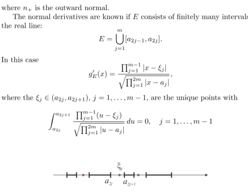
The normal derivatives are known ifEconsists of finitely many intervals on the real line:
E= [m j=1
[a2j−1, a2j].
In this case
g′E(x) =
Qm−1
j=1 |x−ξj| qQ2m
j=1|x−aj| ,
where theξj ∈(a2j, a2j+1),j= 1, . . . , m−1, are the unique points with Z a2j+1
a2j
Qm−1
j=1 (u−ξj) qQ2m
j=1|u−aj|
du= 0, j= 1, . . . , m−1
a2j a2j+1 xj
Figure 3: The position of the pointsξj
Next, let us suppose thatz∈Elies on the outer boundary ofE(i.e. it lies on the boundary of the unbounded component Ω ofC\E), and that outer boundary
is aC2-smooth arc Γ in a neighborhood ofz. In that case the equilibrium density ωE (with respect to arc measure on Γ) of the equilibrium measure is given in terms of the normal derivatives of the Green’s function:
ωE(z) = 1
2π(g−′ (z) +g+′ (z)). (10) This formula should be understood in the sense that if one side of Γ does not belong to Ω (i.e. it belongs toE or to a bounded component ofC\E), then the corresponding normal derivative is considered to be 0 (as the Green’s function is considered to be 0 outside the unbounded component Ω ofC\E). For example, ifE is a Jordan curve (homeomorphic image of a circle), then
ωE(z) = 1
2πg′+(z), (11)
where g′+ is the normal derivative with respect to the outer normal to E. On the other hand, ifE is a Jordan arc (homeomorphic image of a segment), then both derivatives appear in (10). In particular, ifE⊂R, then
ωE(z) = 1
πg′E(z) (12)
because the two normal derivatives are the same.
4 The general Bernstein inequality
The general form of Bernstein’s inequality for sets on the real line were given in [4] and [32]: letE ⊂Rbe a compact set. Then, for algebraic polynomialsPn
of degree at mostn= 1,2, . . ., we have
|Pn′(x)| ≤nπωE(x)kPnkE, x∈Int(E). (13) This is sharp: if x0 ∈ Int(E) is arbitrary, then there are polynomials Pn of degree at mostn= 1,2, . . .such that
|Pn′(x0)|>(1−o(1))nπωE(x0)kPnkE.
Using (12) the inequality (13) can be written in the alternative form:
|Pn′(x)| ≤ngE′ (x)kPnkE, x∈Int(E). (14) Note that in the special caseE= [−1,1] this gives back the original Bernstein inequality (2) becauseg[−1,1]′ (x) = 1/√
1−x2.
Actually, for real polynomials more than (14) is true (see [36]):
Pn′(x) gE′ (x)
2
+n2Pn(x)2≤n2kPnk2E, x∈Int(E), (15) which is the analogue of the beautiful inequality
Pn′(x)p
1−x22
+n2Pn(x)2≤n2kPnk2[−1,1], x∈(−1,1), (16) of G. Szeg˝o [31] and G. Schaake and J. G. van der Corput [30].
5 Markov’s inequality
The classical Markov inequality (3) complements Bernstein’s inequality (2) when we have to estimate the derivative of a polynomial on [−1,1] close to the end- points. What happens if we consider more than one intervals?
LetE =∪mj=1[a2j−1, a2j],a1 < a2<· · ·< a2m, consist of m real intervals.
When we consider the analogue of the Markov inequality for E, actually we have to talk about one-one Markov inequality around every endpoint of E.
Indeed, away from the endpoints (13) is true, therefore there the derivative can be only of orderCn, so ann2rate for the derivative can occur only close to the endpoints, and it is clear that different endpoints play different roles. Letaj be an endpoint ofE, and letEj be the part ofE that lies closer toaj than to any other endpoint. LetMj be the smallest constant for which
kPn′kEj ≤(1 +o(1))Mjn2kPnkE (17) holds, whereo(1) tends to 0 (uniformly in the polynomials Pn) as n tends to infinity. ThisMjdepends on what endpointaj we are considering, and it is the asymptotically best constant in the corresponding local Markov inequality. Its value can be expressed in terms of the normal derivativegE′ of the Green’s func- tiongE. Indeed, around aj this normal derivative behaves like∼1/p
|t−aj|, and the limit
Ωj := lim
t→aj, t∈E
q
|t−aj|gE′ (t)
exists. With it the asymptotic Markov factor can be expressed (see [32]) as Mj= 2Ω2j, j = 1, . . . ,2m.
As an example, consider E = [−b,−a]∪[a, b]. In this case m = 2, a1 =
−b, a2=−a, a3=a, a4=b, and,
gE′ (t) =p |t|
(b2−t2)(t2−a2). Hence,
M1=M4= b
b2−a2, M2=M3= a b2−a2. SinceM1=M4> M2=M3, we obtain that
kPn′k[−b,−a]∪[a,b]≤(1 +o(1))n2 b
b2−a2kPnk[−b,−a]∪[a,b], which is a result of P. Borwein from [11].
As an immediate consequence of the theorem we get the following asymp- totically best possible global Markov inequality:
kPn′kE≤(1 +o(1))n2
1≤j≤2mmax 2Ω2j
kPnkE.
Here theo(1) tends to 0 uniformly in the polynomialsPn asn→ ∞, and this term cannot be dropped. It seems to be a difficult problem to find, on several intervals, for eachnthe best Markov constant for polynomials of degree at most n.
6 M. Riesz and Hilbert’s lemniscate theorem
Let C1 = {z |z| = 1} be the unit circle and Pn an algebraic polynomial of degree at mostn. ThenPn(eit) is a trigonometric polynomial of degree at most n, so by Bernstein’s inequality (1) we have
dPn(eit) dt
≤nmax|Pn|.
The left hand side is|Pn′(eit)ieit|=|Pn′(eit)|, so the previous inequality can be rewritten as
|Pn′(z)| ≤nkPnkC1, z∈C1. (18) This inequality is due to M. Riesz, and was proved in the paper [29] which contained the first proof of Bernstein’s inequality (2) (Bernstein had 2ninstead ofnin (2)).
Riesz’ inequality has been extended to Jordan curves and families of Jordan curves in [23]: ifEis a finite union of disjointC2Jordan curves (homeomorphic images of circles), then for polynomialsPn of degree at most n = 1,2, . . . we have
|Pn′(z)| ≤(1 +o(1))ng′+(z)kPnkE, z∈E, (19) where g′+(z) is the normal derivative of the Green’s function gE taken with respect to the outer normal. Here o(1), which tends to 0 uniformly in Pn as n→ ∞, cannot be dropped. Furthermore, (19) is best possible: ifz0∈E, then there are polynomialsPn6≡0 of degree at mostn= 1,2, . . .for which
|Pn′(z0)| ≥(1−o(1))ng′+(z0)kPnkE.
For the unit circle we haveg′+(z) = 1, so, modulo the factor (1 +o(1)), (19) gives back the original inequality (18) of M. Riesz (which, in general, cannot be dropped in the Jordan curve case).
So far we have not said anything about how to prove the general versions of the classical polynomial inequalities, so let us indicate the proof for (19). The key is to consider lemniscates, i.e. level sets of polynomials. A typical lemniscate is of the form σ = TN−1C1 = {z |TN(z)| = 1}, where TN is a polynomial of some degreeN. We have already mentioned (see (9)) that g′+(z) =|TN′ (z)|/N, so ifE =σand thePn in (19) is of the special form Pn(z) =Rm(TN(z)) with some polynomialRm, thenn=mN, and from Riesz’ inequality applied toRm
we have forz∈σ
|Pn′(z)|=|R′m(TN(z))Tn′(z)| = |Rm′ (TN(z))|N g′+,σ(z)
≤ mkRmkC1N g′+,σ(z) =ng′+,E(z)kPnkE,
which is (19) without the factor (1 +o(1)).
Note that even though this is only a very special case of (19) (the set is a lemniscate and the polynomial is of the special formRm(TN)), a crucial thing has happened in this simple step: although we have started from the unit circle, we got a result on a set that may consist of several components.
The next step is to get rid of the special form Rm(TN) of Pn to get the full (19), but still on a lemniscateE =σ. This is quite subtle, see [23] or [34]
how to do that. The final step is to approximate a union of smooth Jordan curves by lemniscates, which is done by a sharp form of Hilbert’s lemniscate theorem. Hilbert’s lemniscate theorem claims that ifK is a compact set on the plane with connected complement andU is a neighborhood ofK, then there is a lemniscateσthat separatesK andC\U, i.e. it lies withinU but enclosesK.
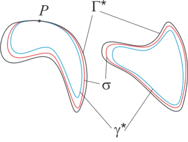
We can reformulate this as follows. Letγj,Γj,j = 1, . . . , m, be Jordan curves (i.e. homeomorphic images of the unit circle),γj lying interior to Γj and the Γj’s lying exterior to one another, and setγ∗=∪jγj, Γ∗=∪jΓj. Then there is a lemniscateσthat is contained in the interior of Γ∗ which also containsγ∗ in its interior, i.e. σseparatesγ∗and Γ∗in the sense that it separates eachγjfrom the corresponding Γj. This is not enough for our approximation, what we need is the following sharpened form (see [23]). Letγ∗ and Γ∗ be twice continuously differentiable in a neighborhood of a pointP where now we assume that they touch each other. We also assume that their curvature atP are different. Then there is a lemniscateσ that separates γ∗ and Γ∗ and touches both γ∗ and Γ∗ atP, see Figure 4. Furthermore,σlies strictly in betweenγ∗and Γ∗ except for the pointP, it has precisely one connected component in between each γj and Γj, j = 1, . . . , m, and these m components are Jordan curves. (Actually, the same statement is true ifγ∗ and Γ∗ touch each other in finitely many points.)
g*
G*
s P
Figure 4: The lemniscateσseparatingγ∗ and Γ∗
Now having settled (19) for lemniscates, the final step in proving (19) for a
system of (C2) Jordan curvesE at a specific point z0 ∈E is to use the sharp form of the Hilbert lemniscate theorem to Γ∗ =E, and to aγ∗ which touches E as in the theorem, and which otherwise lies very close toE. Thisγ∗ can be chosen so close toE that atz0we haveωγ∗(z0)≤(1 +ε)ωE(z0), providedε >0 is given. Then automatically for theσlying in between γ∗ andE we have
g′+,σ(z0)≤g′+,γ∗(z0)≤(1 +ε)g+,E′ (z0), and by theσ-version of (19) we obtain
|Pn′(z0)| ≤(1 +o(1))ng+,σ′ (z0)kPnkσ≤(1 +o(1))n(1 +ε)g′+,E(z0)kPnkE, because kPnkσ ≤ kPnkE by the maximum principle. Since ε > 0 is arbitrary, (19) follows.
The general Bernstein and Markov inequalities ((13) and (17)) can be proven along similar lines using “real lemniscates”, i.e. polynomial inverse images TN−1[−1,1], see [32], [34].
7 Jordan arcs
So far, in the general inequalities we have considered, always one of the normal derivatives of the Green’s function gave the (asymptotically) best Bernstein- factors, and the Markov-factors have also been expressed in terms of them. In some sense this was accidental, it is due to either a symmetry (whenE ⊂R) or to an absolute lack of symmetry (whenE was a Jordan curve for which the two sides ofE, the exterior and interior of E, play absolutely different roles).
The case of Jordan arcs (which have not been considered so far), show the true nature of these inequalities.
So let E be a Jordan arc, i.e. a homeomorphic image of a segment. We assume C2+ (a little more than C2) smoothness of E. As has already been discussed in Section 2,E has two sides, and every point z ∈E different from the endpoints of E gives rise to two different points z± on the two sides and formula (8) holds.
Now the Bernstein inequality onEtakes the form (forz∈Ebeing different from the two endpoints ofE)
|Pn′(z)| ≤(1 +o(1))nmax g−′ (z), g′+(z)
kPnkE, (20) whereo(1) tends to 0 uniformly inPn asn→ ∞, see [22]. This is best possible, one cannot write anything smaller than max(g′−(z), g′+(z)) on the right. The first result in this direction was in the paper [21] by B. Nagy and S. Kalmykov which contains (20) for analytic arcs.
To appreciate the strength of (20) (or that of (19)) let us mention that the smooth Jordan arc (curve) in it can be arbitrary, and a general smooth Jordan arc (curve) can be pretty complicated, see for example, Figure 5.
Figure 5: A “wild” Jordan arc
As for Markov’s inequality, let now wbe one of the endpoints ofE, and let E˜ be the part of E that is closer to z than to the other endpoint of E. As z→w, the common limits
Ωw= lim
z→w, z∈E
p|z−w|g−′ (z) = lim
z→w, z∈E
p|z−w|g′+(z)
exist, and with it we have the Markov-inequality aroundw(see [22]):
kPn′kE˜ ≤(1 +o(1))n22Ω2wkPnkE, (21) and this is best possible in the sense that one cannot write a smaller number than 2Ω2won the right.
8 Higher derivatives
The Markov inequality (3) can be iterated to get for anyk = 1,2, . . . for the k-th derivative
kPn(k)k[−1,1] ≤n2(n−1)2· · ·(n−k+ 1)2kPnk[−1,1].
However, this is not sharp, the correct bound was proven as early as 1892 by V.
A. Markov [20], the brother of A. A. Markov:
kPn(k)k[−1,1]≤ n2(n2−12)(n2−22)· · ·(n2−(k−1)2)
1·3· · ·(2k−1) kPnk[−1,1]. (22) This turns into an equality for the Chebyshev polynomialsPn(x) = cos(narccosx).
The corresponding inequality for several intervals or for a Jordan arc is not known and it is pretty hopeless, but we do have the asymptotically sharp Markov-inequality which involves the factor 1/1·3· · ·(2k−1) = 1/(2k−1)!!
from (22). For example, (17) for higher derivatives takes the form kPn(k)kEj ≤(1 +o(1))n2k (2Ω2j)k
(2k−1)!!kPnkE
while (21) has the extension
kPn(k)kE˜≤(1 +o(1))n2k (2Ω2w)k
(2k−1)!!kPnkE,
and both of these are best possible (no smaller number can be written on the right).
9 Almost everywhere results
LetE⊂Rbe an arbitrary arbitrary compact set of positive linear measure. As early as 1916 J. Privalov proved [26] that for everyε >0 there is aCεsuch that
|Pn′(x)| ≤CεnkPnkE
for all x∈ E with the exception of a set of measure < ε. A sharper form is contained in [35, Corollary 2.3]: define forx∈E
b
ωE(x) = lim
δ→0ωEδ(x),
whereEδ is the δ-neighborhood of E (the limit exists, forωEδ(x) decreases as δincreases). By Fatou’s lemma
Z b
ωEδ(x)dx≤1.
Now if x ∈ E is any point (not just interior point), then for any algebraic polynomialPn of degree at mostn= 1,2, . . . we have
|Pn′(x)| ≤nπωbE(x)kPnkE. (23) Conversely, if γ < πωbE(x), then there are algebraic polynomials Pn 6≡ 0 of arbitrarily large degreensuch that
|Pn′(x)| ≥nγkPnkE. (24) These show that in Privalov’s theorem one can choose, for example, Cε = π/ε.
10 Local results
Let againE⊂R. We shall now address the problem when
|Pn′(x0)| ≤CnkPnkE
is true at a given point x0 with some constant C independent of Pn and n.
Without loss of generality we may choose x0 = 0, so the question is what structural properties ofE guarantee
|Pn′(0)| ≤CnkPnkE. (25)
V. Andrievskii proved in [3] that (25) is true if and only if
gE(z)≤C|z|, z∈C, (26) i.e. if and only if the Green’s functiongE is Lip 1 at the point 0. Furthermore, if (26) is true, then the normal derivative
g′E(0) = lim
t→0
gE(it) t exists, and it is the asymptotically bestC in (25).
It is quite remarkable, that (25) is equivalent to a similar inequality for higher derivatives (see [37]): Ifk≥2 fixed, then (25) is true if and only if
|Pn(k)(0)| ≤CnkkPnkE (27) holds (naturally, with a possibly different constantC than in (25)). Note that neither direction of the equivalence (25)⇔(27) is trivial, even not⇒, for (25) cannot be iterated since the local Bernstein inequality in it is known only at the single point 0.
Another somewhat surprising fact is that for (25) to hold the set does not need to be thick in measure-theoretical sense, namely
there is anE of Lebesgue-measure 0 for which (25) is true. (28)
A proof of this fact follows from the equivalence of (25) and (26), from [33, Corollary 5.2] and from [12, Corollary 1.12].
However, the set E must be thick at 0 in potential-theoretical sense as is shown by the following characterization of (26). For that we need the notion of logarithmic capacity. Recall that
gE(z)∼log|z|+ const as z→ ∞, and in fact the limit
z→∞lim(log|z| −gE(z)) exists, and we set
log cap(E) := lim
z→∞(log|z| −gE(z)).
For example, the capacity of a line segment of lengthℓisℓ/4, and the capacity of a circle/disk of radiusrisr. IfE is connected and Φ is a conformal map of the complement onto the exterior of the unit disk, then around∞
Φ(z) = z
cap(E)+c0+c−1
z +c−2
z2 +· · ·.
e2-k (1- )e 2-k 2-k 0
Ek
Figure 6: The depiction of the setsEk
With some fixed 0< ε <1/3 define nowIk= [0,2−k], Ek = (E∩Ik)∪[0, ε2−k]∪[(1−ε)2−k,2−k],
and similarly define Ik and Ek for negative k by using |k| in the just given formulae.
Define also the capacitary defect
θk= (cap(Ik)−cap(Ek))/cap(Ik) = 2|k|+2(cap(Ik)−cap(Ek)).
With this the characterization of the Lip 1 property reads as (see [12, Theorem 11])
gE(z)≤C|z| ⇐⇒ X
k
θk<∞.
11 Bernstein’s approximation theorem
The aforementioned results are connected with the famous theorem of S. N.
Bernstein on the rate of polynomial approximation of|x|. Let En(f(x), E) = inf
deg(Pn)=nkf(x)−Pn(x)kE
be the rate of the best approximation off(x) onE by polynomials of degreen.
Bernstein’s result says (see [8]) that
n→∞lim nEn(|x|,[−1,1]) =σ
exists, finite and positive. The value of σ is still not known today. Later Bernstein extended his result ([9], [10]): ifp >0 is not an even integer, then
n→∞lim npEnp(|x|p,[−1,1]) =σp, (29) and he also considered the non-symmetric case: ifa <0< b, then
n→∞lim npEn(|x|p,[a, b]) =p
|a|b·σp, with the sameσp as in (29).
R. K. Vasiliev considered approximation of |x|p on an arbitrary compact E⊆R. His main result is that if 0∈Int(E), then
n→∞lim npEn(|x|p, E) = σp
gE′ (0). (30)
This result is from [38], where it is stated in a completely different form and it is one of the two theorems in that book. Unfortunately, the second theorem is not correct (contradicts (28)), and it is difficult to tell what went wrong in the close to 160 pages of reasonings. The form (30) of Vasiliev’s theorem was given in [33, Theorem 10.5] along with a relatively short, about 5 pages proof.
There is also an analogue of (28): ifpis not an even integer, then there is a setE of Lebesgue-measure zero for which
lim inf
n→∞ npEn(|x|p, E)>0.
See [33, Corollary 10.4].
On the other hand, a recent result of V. Andrievskii (see [1], [2]) claims that (forpnot an even integer)
lim inf
n→∞ npEn(|x|p, E)>0 if and only if
gE(z)≤C|z|,
so ≥ c/np rate of polynomial approximation of |x|p is equivalent to the local Bernstein-inequality (25) which in turn is equivalent to the Lip 1 property of the Green’s function at the point 0.
12 Endpoint results
The preceding results have an analogue for endpoints that will be proven in [37].
In fact, suppose thatE ⊂Ris compact, 0∈E, but (−a,0)∩E =∅for some a >0 (0 is an “endpoint” ofE). At such points we have the complete analogue of what were discussed above: for a fixedk≥2 and forp >0 not an integer the following are equivalent.
• |Pn′(0)| ≤Cn2kPnkE,
• |Pn(k)(0)| ≤Cn2kkPnkE,
• gE(z)≤C|z|1/2,
• P
k>0θk<∞,
• lim infn→∞n2pEn(|x|p, E)>0.
As before, here theC may be different at different occurrences.
References
[1] V. Andrievskii, Polynomial approximation of piecewise analytic functions on a compact subset of the real line,J. Approx. Theory,161(2009), 634–644.
[2] V. Andrievskii, Polynomial approximation on a compact subset of the real line,J. Approx. Theory,230(2018), 24–31.
[3] V. Andrievskii, Bernstein polynomial inequality on a compact subset of the real line,J. Approx. Theory,245(2019), 64–72.
[4] M. Baran, Bernstein type theorems for compact sets in Rn, J. Approx.
Theory,69(1992), 156–166.
[5] A. D. Baranov, Embeddings of model subspaces of the Hardy class: compact- ness and Schatten-von Neumann ideals. (Russian), Izv. Ross. Akad. Nauk Ser. Mat.,73(2009), 3–28; translation inIzv. Math.,73(2009), 1077–1100.
[6] J. Beck, Flat polynomials on the unit circle - note on a problem of Little- wood,Bull. London Math. Soc.,23(1991), 269–277.
[7] S. N. Bernstein, Sur l’ordre de la meilleure approximation des fonctions continues par les polynˆomes de degr´e donn´e, M´emoires publi´es par la Classe des Sciences del l’Acad´emie de Belgique,4, 1912.
[8] S. N. Bernstein, Sur la meilleure approximation de |x| par des polynomes des degr´es donn´es,Acta Math.,37(1914), 1–57.
[9] S. N. Bernstein, On the best approximation of|x|pby means of polynomials of extremely high degree, Izv. Akad. Nauk SSSR, Ser. Mat. 2(1938), 160–
180. Reprinted in S. N. Bernstein Collected Works, Vol. 2, pp. 262–272.
Izdat. Nauk SSSR, Moscow, 1954 (Russian).
[10] S. N. Bernstein, On the best approximation of|x−c|p, Dokl. Akad. Nauk SSSR, 18(1938), 379–384. Reprinted in S. N. Bernstein Collected Works, Vol. 2, pp. 273–260. Izdat. Nauk SSSR, Moscow, 1954 (Russian).
[11] P. Borwein, Markov’s and Bernstein’s inequalities on disjoint intervals, Canad. J. Math.33(1981), 201–209.
[12] L. Carleson and V. Totik, H¨older continuity of Green’s functions,Acta Sci.
Math.,70(2004), 557–608.
[13] Q. Chen, C. Miao and Z. Zhang, A new Bernstein’s inequality and the 2D dissipative quasi-geostrophic equation,Comm. Math. Phys.,271(2007), 821–838.
[14] T. Erd´elyi, The phase problem of ultraflat unimodular polynomials: the resolution of the conjecture of Saffari,Math. Ann.,321(2001), 905–924.
[15] F. Filbir and H. N. Mhaskar, A quadrature formula for diffusion polyno- mials corresponding to a generalized heat kernel, J. Fourier Anal. Appl., 16(2010), 629-657.
[16] J. Krieger and K. Nakanishi, Large time decay and scattering for wave maps,Dyn. Partial Differ. Equ.,5(2008), 1–37.
[17] D. S. Lubinsky, Some recent methods for establishing universality limits, Nonlinear Anal., 71(2009), 2750–2765.
[18] H. L. Montgomery,Ten lectures on the interface between analytic number theory and harmonic analysis, CBMS Regional Conference Series in Math- ematics, 84.Published for the Conference Board of the Mathematical Sci- ences, Washington, DC; by the American Mathematical Society, Providence, RI, 1994.
[19] A. A. Markov, On a question by D. I. Mendeleev,Zap. Imp. Akad. Nauk SPb.,62(1890), 1–24. (Russian)
[20] V. A. Markov, On functions of least deviation from zero in a given interval (1892). Appeared in German as ” ¨Uber Polynome, die in einem gegebenen Intervalle m¨oglichst wenig von Null abweichen”.Math. Ann.,77(1916), 213–
258.
[21] B. Nagy and S. Kalmykov, Polynomial and rational inequalities on analytic Jordan arcs and domains,J. Math. Anal. Appl.,430(2015), 874–894.
[22] B. Nagy, S. Kalmykov and V. Totik, Bernstein- and Markov-type inequal- ities for rational functions,Acta Math.,219(2017), 21–63
[23] B. Nagy and V. Totik, Sharpening of Hilbert’s lemniscate theorem, J.
D’Analyse Math.,96(2005), 191–223.
[24] P. Oswald, Optimality of multilevel preconditioning for nonconforming P1 finite elements,Numer. Math.,111(2008), 267–291.
[25] I. Pesenson and A. I. Zayed, Paley-Wiener subspace of vectors in a Hilbert space with applications to integral transforms,J. Math. Anal. Appl., 353(2009), 566–582.
[26] J. Privalov, Sur la convergence des s´eries trigonom´etriques conjug´ees, Comptes Rendus de l’Aced´emie des Sciences, Paris,162(1916), 123–126.
[27] T. Ransford,Potential Theory in the Complex plane, Cambridge University Press, Cambridge, 1995.
[28] Sz. Gy. R´ev´esz, N. N. Reyes and G. A. M. Velasco, Oscillation of Fourier transforms and Markov-Bernstein inequalities, J. Approx. Theory, 145(2007), 100–110.
[29] M. Riesz, Eine trigonometrische Interpolationsformel und einige Un- gleichungen f¨ur Polynome, Jahresbericht der Deutschen Mathematiker- Vereinigung,23(1914), 354–368.
[30] G. Schaake and J. G. van der Corput, Ungleichungen f¨ur Polynome und trigonometrische Polynome,Compositio Math.,2(1935), 321-361.
[31] G. Szeg˝o, ¨Uber einen Satz des Herrn Serge Bernstein, Schriften K¨onigs- berger Gelehrten Ges. Naturwiss. Kl.,5(1928/29), 59–70.
[32] V. Totik, Polynomial inverse images and polynomial inequalities, Acta Math.,187(2001), 139–160.
[33] V. Totik,Metric properties of harmonic measures, Memoirs of the American Mathematical Society,184, number 867, 2006
[34] V. Totik, The polynomial inverse image method, Approximation The- ory XIII: San Antonio 2010, Springer Proceedings in Mathematics, 13, M.
Neamtu and L. Schumaker (eds.), 345–367.
[35] V. Totik, Bernstein and Markov type inequalities for trigonometric polyno- mials on general sets,Int. Math. Res. Not., IMRN 2015, no. 11, 29863020.
[36] V. Totik, Bernstein-type inequalities,J. Approx. Theory,164(2012), 1390–
1401.
[37] V. Totik, Reflections on a theorem of V. Andrievskii (in preparation) [38] R. K. Vasiliev,Chebyshev Polynomials and Approximation Theory on Com-
pact Subsetc of the Real Axis, Saratov University Publishing House, 1998.
Department of Mathematics and Statistics University of South Florida
4202 E. Fowler Ave, CMC342 Tampa, FL 33620-5700, USA and
Bolyai Institute
MTA-SZTE Analysis and Stochastics Research Group University of Szeged
Szeged
Aradi v. tere 1, 6720, Hungary totik@mail.usf.edu