arXiv:1802.01558v2 [math.PR] 9 Feb 2018

RANDOM WALK ON THE RANDOMLY-ORIENTED MANHATTAN LATTICE

SEAN LEDGER, BÁLINT TÓTH, AND BENEDEK VALKÓ

Abstract. In the randomly-oriented Manhattan lattice, every line inZ^d is assigned a uniform random direction. We consider the directed graph whose vertex set is Z^d and whose edges connect nearest neighbours, but only in the direction fixed by the line orientations. Random walk on this directed graph chooses uniformly from the d legal neighbours at each step. We prove that this walk is superdiffusive in two and three dimensions. The model is diffusive in four and more dimensions.

1. Introduction, notation and results

To define the randomly-oriented Manhattan lattice, let E ={±e₁,±e₂, . . . ,±e_d} be the canonical unit vectors inZ^d and let

U_i :={x∈Z^d:hx, e_ii= 0}, i∈ {1,2, . . . , d}.

These (d−1)-dimensional subspaces of Z^d allow us to uniquely index the lines in Z^d that are parallel to a canonical unit vector as

V(i, x) :={x+te_i :t ∈Z}, for i∈ {1,2, . . . , d}, x∈U_i.

Assign to each line V(i, x), x ∈ Ui the direction ei or −ei with probability 1/2 each, independently of each other. For eachx∈Z^d we denote byω(i, x)the chosen direction corresponding to the line{x+te_i :t∈Z}. Note that ω(i, x) =ω(i, x− hx, e_ii).

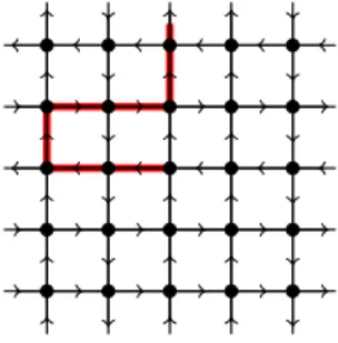
We study a continuous-time nearest neighbor random walk on Z^d in the random environment ω(i, x). The walker takes steps at rate d, and if it is at x ∈ Z^d then its next position is chosen uniformly from the set {x+ω(i, x),1 ≤ i ≤ d}. (See Figure 1.1.) Our main object of interest is the mean-square displacement

E(t) :=E[|Xt|²], t≥0,

whereX_t denotes the position of the walker at time t. Notice that the model is trivial whend = 1.

We analyse the asymptotics of E by applying theresolvent method. The method was introduced in [3, 5, 11] to give diffusivity estimates for a tracer particle in a Gaussian drift field, respectively, for a second class particle in the asymmetric exclusion process onZand Z². Later the method was used in [8, 10] to study the long-time behaviour of self-repelling diffusions pushed by the negative gradient of their local time and diffusion driven by the curl-field of the Gaussian Free Field in 2 dimensions.

In this note we show how the method transfers to the Manhattan lattice to prove superdiffusivity of the random walk in d = 2 and d = 3. The method employed is very similar to that of [8, 10]. However, this particular model has some interest and

1

arXiv:1802.01558v2 [math.PR] 9 Feb 2018

Figure 1.1. A typical initialisation of the random line directions in the Manhattan lattice with a legal path for the walker (red).

notoriety (see e.g. [1, 2]) and the authors have been repeatedly requested to spell out the full proof.

Our main theorem provides bounds on the Laplace transform of E E(λ) =b

ˆ ∞ 0

e^−λtE(t)dt, asλ →0.

Theorem 1.1. There exists finite positive constants C and λ0 such that for all 0 <

λ < λ₀ we have

C⁻¹λ^−9/4 ≤E(λ)b ≤Cλ^−5/2 if d= 2, and C⁻¹λ⁻²log log(λ⁻¹)≤E(λ)b ≤Cλ⁻²log(λ⁻¹) if d= 3.

The bounds in Theorem 1.1 are time-averaged, they should correspond to behaviour t^5/4 . E(t) . t^3/2 in two dimensions and tlog logt . E(t) . tlogt in three dimen- sions. In fact, the upper bounds on E(t) can be transferred from those on E(λ)b by [8, Lem. 1]. The lower bounds onE(λ)b do not transfer pointwise without some additional information on E(t), but they do give the corresponding growth rates for the Cesàro average ¹_t´_t

0 E(s)ds.

In four and higher dimensions the random walk is known to be diffusive, in fact [4, 9]

proves central limit theorem for the random walk both in the quenched and annealed environment.

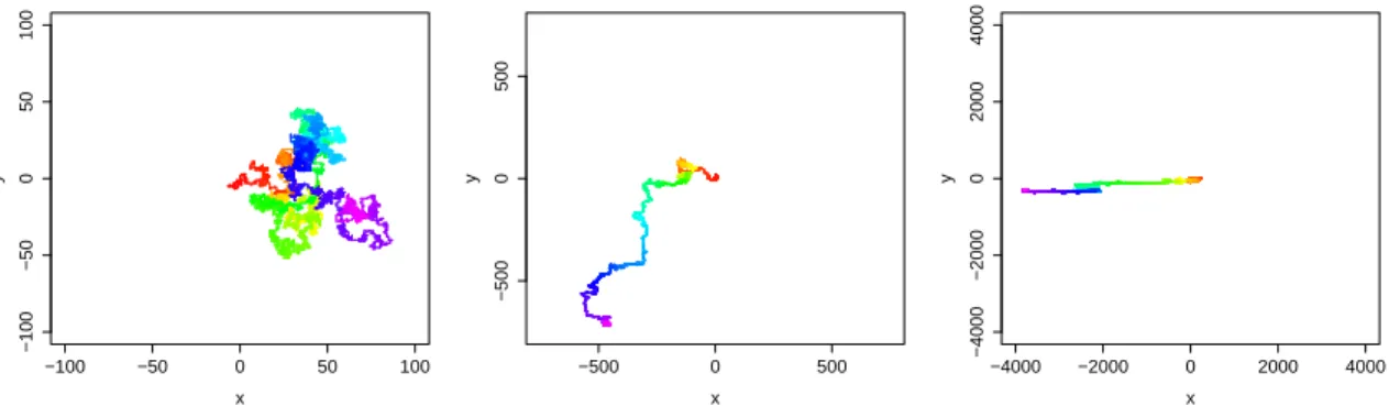
The bounds on the growth rates in Theorem 1.1 are not sharp. A non-rigorous Alder–Wainwright type scaling argument (see e.g. [10]) suggests that the true behavior is E(t) t^4/3 for d = 2, and E(t) t(logt)^1/2 for d = 3. A heuristic explanation for the superdiffusive behaviour is that when the walk enters a region with many lines oriented in the same direction, it tends to follow a long and relatively straight path in that direction (see Figure 1.2).

Random walk on the randomly-oriented Manhattan lattice is closely related to the Matheron–de Marsily (MdM) model, originally introduced in [6]. In the MdM model, one dimension has fixed uniformly chosen random line directions as in the Manhattan lattice, but all other components are undirected. At each jump time the walker choses uniformly one of the d lines going through its position. If the chosen line is one of the directed ones then the walker takes a step in that direction, otherwise it choses one of the two neighbours on the line randomly.

−100 −50 0 50 100

−100−50050100

x

y

−500 0 500

−5000500

x

y

−4000 −2000 0 2000 4000

−4000−2000020004000

x

y

Figure 1.2. Realisation for the first 10,000 steps: the left shows simple ran- dom walk on Z², the centre shows random walk on a randomly-oriented Man- hattan lattice (orientations not shown) and the right shows the MdM model with orientations in the x-component. Time is indexed by colour.

The MdM model is well-studied [1, 2], and its mean-square displacement can be analysed exactly, giving scaling E(t)t^3/2 when d= 2 and E(t)tlogt when d= 3.

There is a natural way to interpolate between the MdM and the Manhattan lattice model: suppose thatdfix≥ 1of the dimensions of the lattice are directed and dfree are undirected, where dfix+dfree =d. Then dfix = 1 gives the MdM model, while dfix =d gives the Manhattan lattice model. This offers no new models in two dimensions and all the intermediate models can be shown to be diffusive in four and higher dimension.

There is, however, one potentially interesting case when d= 3 and d_fix = 2. In Section 4 we show that for this model we have

C⁻¹λ⁻²p

logλ⁻¹ ≤E(λ)b ≤Cλ⁻²log(λ⁻¹), (1.1)

provided thatλis small enough. Non-rigorous scaling arguments suggests that the true growth isE(t)t(logt)^2/3 in this case.

Notation and outline of the proof. We will proceed by analysing the environment of randomly oriented lines as seen from the position of the random walker. Denote the set of possible environments by

Ω =

d

O

i=1

O

x∈U_i

{−1,1}.

For a given x ∈ U_i the set {−1,1} corresponds to {−e_i, e_i}. For an ω ∈ Ω we denote the coordinates (with a slight abuse of notation) byω(i, x), 1≤i≤d,x∈U_i.

Letτ_i : Ω→Ωbe the translation of the environment bye_i and τ_i⁻¹ its inverse. These act on the coordinates as

τiω(i, x) =τ_i⁻¹ω(i, x) =ω(i, x) and

τ_iω(j, x) =ω(j, x+e_i), and τ_i⁻¹ω(j, x) =ω(j, x−e_i), for j 6=i.

The joint distribution of the environment is given by the product measure

(1.2) π =

d

O

i=1

O

x∈U_i

µ_i,x,

where µ_i,x is the uniform measure on {−1,1}. Note that π is invariant with respect to the translations τ_i, τ_i⁻¹. For functions f, g ∈ L²(Ω, π) we will use the notation (f, g)_π =´

f gdπ.

Let η_t∈Ω be the environment seen from the position of the random walker at time t. Thenη_t is a Markov process, and its generator can be expressed as follows:

Gf(ω) :=

d

X

i=1

1 +ω(i,0)

2 f(τ_iω) + 1−ω(i,0)

2 f(τ_i⁻¹ω)−f(ω)

. (1.3)

Note that if η = (η_t)t≥0 is the environment process viewed from the walker and X = (X_t)t≥0 is the position of the walker, then

(1.4) η_t(i, x) = η₀(i, x−X_t).

An important observation is that π is an invariant measure for η_t. It can be checked that the adjoint ofG is given by

G^∗f(ω) =

d

X

i=1

1−ω(i,0)

2 f(τ_iω) + 1 +ω(i,0)

2 f(τ_i⁻¹ω)−f(ω)

,

and hence the symmetric and antisymmetric parts ofG are given by S = ¹₂(G+G^∗) Sf(ω) = ¹₂

d

X

i=1

(f(τ_iω) +f(τ_i⁻¹ω)−2f(ω)), (1.5)

A= ¹₂(G−G^∗) Af(ω) =

d

X

i=1

ω(i,0)(f(τ_iω)−f(τ_i⁻¹ω)).

(1.6)

Notice thatS is the generator of a the environment process as seen from a symmetric simple random walk onZ^d.

We now sketch the basic strategy of the resolvent method. By symmetry we have E(t) =E|X_t|² =d·E|X_t¹|² whereX_t¹ is the first coordinate ofX_t. Observe that(X_t¹, η_t) is also a Markov process with a generator

Ge1f(z, ω) = 1 +ω(1,0)

2 f(z+ 1, τ1ω) + 1−ω(1,0)

2 f(z−1, τ₁⁻¹ω)−f(z, ω), and that with f(z, ω) =z we get Ge₁f(z, ω) =ω(1,0). From this it follows that

X_t¹ =M_t+ ˆ _t

0

φ(η_s)ds,

where φ(ω) = ω(1,0), and M_t is a martingale with E[M_t²] = ct with a constant c.

Introduce the quantity E_G(t) :=E

hˆ t 0

φ(η_s)ds2i

= 2 ˆ t

0

(t−s)E[φ(η₀)φ(η_s)]ds.

From the inequality ¹₂a²−b² ≤(a+b)² ≤2a²+2b²and the fact thatE[M_t²] =ctit follows that superlinear upper and lower bounds on E_G(t)² (or the corresponding bounds on its Laplace transform) imply similar bounds (with different constants) onE[|X_t¹|²], and hence E[|X_t|²] as well. (In fact, it can be shown that E[|X_t¹|²] = E[M_t²] +E_G(t), but this is not needed for us.) This means that if we give upper and lower bounds onEb_G(λ) that grow faster thanλ⁻² as λ → 0, then these bounds will hold for E(λ)b as well, up to constants. Hence it is enough to estimateEb_G.

From the definition ofEGit follows thatEbG(λ) = 2λ⁻²(φ,(λ−G)⁻¹φ)π. The resolvent method relies on the following variational representation of(φ,(λ−G)⁻¹φ)π:

(φ,(λ−G)⁻¹φ)_π = sup

ψ∈L²(Ω,π)

n

2(φ, ψ)_π−(ψ,(λ−S)ψ)_π −(Aψ,(λ−S)⁻¹Aψ)_πo . (1.7)

(A derivation of this formula can be found in [7].) Since the right hand side of (1.7) is a supremum, evaluating the expression2(φ, ψ)_π−(ψ,(λ−S)ψ)_π−(Aψ,(λ−S)⁻¹Aψ)_π for a given ψ ∈ L²(Ω, π) will give a lower bound on (φ,(λ−G)⁻¹φ)_π, and hence on E(λ). The lower bounds in Theorem 1.1 will follow from careful choices of the testb function ψ. The detailed proof is carried out in Section 2. The same idea is used for the lower bound for the intermediate MdM model withd_fix= 2 and d_free = 1, the proof is presented in Section 4.

The upper bounds are easier to obtain. Note that because S is self-adjoint, the term (Aψ,(λ−S)⁻¹Aψ)_π is nonnegative. Dropping it from the expression inside the supremum in (1.7) thus gives the following upper bound:

(φ,(λ−G)⁻¹φ)π ≤ sup

ψ∈L²(Ω,π)

2(φ, ψ)π−(ψ,(λ−S)ψ)π = (φ,(λ−S)⁻¹φ)π.

Since S is the generator of the environment process as seen from a symmetric simple random walk, (φ,(λ −S)⁻¹φ)_π can be computed directly, which leads to the upper bounds onEbG(λ). This is demonstrated in Section 3.

Acknowledgements. BT was supported by EPSRC (UK) Established Career Fellow- ship EP/P003656/1 and by OTKA (HU) K-109684. BV was partially supported by the NSF award DMS-1712551 and the Simons Foundation.

2. Proof of lower bound in Theorem 1.1

Our goal will be to find an appropriate test function ψ ∈L²(Ω, π) where the expres- sion inside the supremum in (1.7) can be evaluated, and is sufficiently large. We will look for the test function in the form

(2.1) ψ(ω) := X

x∈U1

u(x)ω(1, x),

where u ∈ L²(U₁) is an even real function that could also depend on λ. The precise form ofu will be stated later in this section.

We will start with some explicit computations involving the terms in (1.7). In the following we will use the notation

∇⁺_i f(x) :=f(x+e_i)−f(x), ∇_if(x) :=f(x+e_i)−f(x−e_i).

Lemma 2.1 (Preliminary calculations). With ψ defined as in (2.1) we have:

(i) (φ, ψ)_π =u(0), (ψ, ψ)_π =kuk²₂, (ii) (ψ, Sψ)_π =−Pd

i=2k∇⁺_i uk²₂, (iii) Aψ(ω) =−Pd

i=2

P

x∈U1ω(i,0)ω(1, x)∇_iu(x), (iv) Suppose that for fixed i6=j we have

ζ(ω) = X

x∈U_i

X

y∈U_j

v(x, y)ω(i, x)ω(j, y) where P

x,yv(x, y)² <∞. Then Sζ(ω) = 1

2 X

x,y

(v(x+e_j, y) +v(x−e_j, y)−2v(x, y))ω(i, x)ω(j, y)

+1 2

X

x,y

(v(x, y+ei) +v(x, y−ei)−2v(x, y))ω(i, x)ω(j, y)

+1 2

X

k6=i,j

X

x,y

(v(x+e_k, y+e_k) +v(x−e_k, y−e_k)−2v(x, y))ω(i, x)ω(j, y) (2.2)

Proof. The proof of (i) follows directly from the fact that ω(1, x) are i.i.d. mean zero and variance 1 random variables.

To prove (ii) first note that ψ(τ₁ω) = ψ(τ₁⁻¹ω) = ψ(τ), and thus (after rearranging the terms) we get

Sψ(ω) = 1 2

d

X

i=2

X

x∈U_i

(u(x+e_i) +u(x−e_i)−2u(x))ω(1, x).

Hence, after a simple rearrangement of the terms we get (ψ, Sψ)π = 1

2

d

X

i=2

X

x∈U_i

(u(x+ei) +u(x−ei)−2u(x))u(x)

=−

d

X

i=2

X

x∈Ui

(u(x+e_i)−u(x))² =−

d

X

i=2

k∇⁺_i uk²₂.

Both (iii) and (iv) follow from the definitions after some algebraic manipulations and

careful book-keeping.

Fourier representation. Forf :Z^d →R, denote its Fourier transform by f(p) :=b X

x∈Z^d

e^ip·xf(x) p∈T^d, (2.3)

withibeing the imaginary unit andT the torus on[0,2π). (Although we use the same notation for the Laplace transform, it will not cause any confusion.) For anf :U_j →R

we definef(p)b by first extendingf toZ^dby setting it equal to zero outsideU_j and then taking the Fourier transform. This is the same as using (2.3), but with a summation only onU_j. Note that iff :U_j →Rthenf(p)b does not depend onp_j, thejth coordinate of p.

The Fourier transform of a function c:Z^d×Z^d→R is defined as bc(p, q) = X

x,y∈Z^d

e^i(p·x+q·y)c(x, y) p, q ∈T^d.

We can extend this definition to functions of the formc:U_i×U_j →R as in the single variable case.

By Parseval’s formula if f :U_i →R is in L²(U_i) then kfk² = 1

(2π)^d ˆ

T^d

|f(p)|ˆ ²dp, and similarly, ifc:Ui×Uj →Rthen

kck² = X

x∈U_i

X

y∈U_j

c(x, y)² = 1 (2π)^2d

ˆ

T^d

ˆ

T^d

|ˆc(p, q)|²dpdq.

For anu:U1 →R and j 6= 1 we have

∇[⁺_ju(p) = (e^−ipj−1)bu(p).

Note that|e^−it−1|² = 4 sin²(₂^t). For p∈T^d let d(p) =b

d

X

j=1

4 sin²(^p₂^j),

and definep^−j =p−p_je_j as the vector obtained from pby replacing its jth coordinate with 0. Then with ψ defined as in (2.1) we have

(ψ,(λ−S)ψ)_π = 1 (2π)^d

ˆ

T^d

λ+d(pb ⁻¹)

|bu(p)|²dp.

(2.4)

Now suppose thatζ is defined as in part (iv) of Lemma 2.1. According to the lemma, we can express Sζ(ω) as P

x∈Ui

P

y∈Ujv^∗(x, y)ω(i, x)ω(j, y) where v^∗ can be read off from (2.2). From this the Fourier transform of v^∗ can be expressed as follows:

bv^∗(p, q) = 1 2

(

(e^ipj +e^−ipj −2) + (e^iqi+e^−iqi −2) + X

k6=i,j

(e^i(pk+qk)+e^−i(pk+qk)−2) )

bv(p, q)

=−1

2d(pb ⁻ⁱ+q^−j)bv(p, q).

This also shows that(λ−S)⁻¹ζ(ω)can be expressed asP

x∈U_i

P

y∈U_js(x, y)ω(i, x)ω(j, y) with

bs(p, q) =

λ+ ¹₂d(pb ⁻ⁱ+q^−j)−1

bv(p, q).

By Lemma 2.1 we can express Aψ(ω) =

d

X

i=2

X

x∈U_i

X

y∈U₁

v_i(x, y)ω(i, x)ω(1, y) where

v_i(x, y) =−1{x= 0}∇_iu(y), and bv_i(p, q) = (e^iqi −e^−iqi)bu(q).

This leads to the identity

(Aψ,(λ−S)⁻¹Aψ)_π = 1 (2π)^2d

ˆ

T^d

ˆ

T^d d

X

i=2

4 sin²(q_i)

λ+¹₂d(pb ⁻ⁱ+q⁻¹)−1

|bu(q)|²dpdq.

(2.5)

The proceeding integral inequalities follow from simple calculus, comparing sin²(x/2) tox² on(−π, π).

Lemma 2.2. If d= 2 then for all λ >0 and p∈T² we have 1

(2π)^d ˆ

T^d

λ+ ¹₂d(qb ⁻²+p⁻¹)⁻¹

dp≤Cλ^−1/2, (2.6)

where C is a finite constant. If d= 3 then for all p∈T³ and 0< λ≤1/3 we have 1

(2π)^d ˆ

T^d

λ+ ¹₂d(qb ⁻²+p⁻¹)−1

dq ≤C|log(λ+ ¹₂sin²(^p₂²))|, (2.7)

where C is a finite constant.

Estimating(φ,(λ−G)⁻¹φ)π usingψ. Our goal is to give a lower bound on2(φ, ψ)π− (ψ,(λ−S)ψ)_π−(Aψ,(λ−S)⁻¹Aψ)_π when ψ is of the form (2.1), this will also give a lower bound for(φ,(λ−G)⁻¹φ)_π.

By the inverse Fourier formula we have (φ, ψ)_π =u(0) = 1

(2π)^d ˆ

T^d

bu(p)dp.

(2.8)

We assumed thatu is even, hence u(p)b is real.

Using the expression (2.5) for (Aψ,(λ−S)⁻¹Aψ)_π and the bounds of Lemma 2.2 we get that

(Aψ,(λ−S)⁻¹Aψ)π ≤ C (2π)^d

ˆ

T^d

λ^−1/2sin²(p2)|u(p)|b ²dp for d= 2 (2.9)

and

(Aψ,(λ−S)⁻¹Aψ)_π

≤ C (2π)^d

ˆ

T^d 3

X

j=2

|log(λ+¹₂sin²(^p₂^j))|sin²(p_j))|bu(p)|²dp for d= 3, (2.10)

if0< λ≤1/3. Now we have all the ingredients to prove the lower bounds in Theorem 1.1.

Proof of the lower bound for d= 2 in Theorem 1.1. Ifd = 2 then (2.4), (2.8) and (2.9) show that for a ψ of the form (2.1) we have

2(φ, ψ)_π−(ψ,(λ−S)ψ)_π −(Aψ,(λ−S)⁻¹Aψ)_π

≥ 1 (2π)²

ˆ

T²

2bu(p)−

λ+d(pb ⁻¹)

|bu(p)|²−Cλ^−1/2sin²(p2)|u(p)|b ² dp, with a fixed constantC > 0.

The integral achieves its maximum for the choice

u(p) =b 1

λ+d(pb ⁻¹) +Cλ^−1/2sin²(p₂),

note that this is real, bounded and only depends onp₂, thus it corresponds to a function u:U₁ →R that satisfies our assumptions. The value of the integral for this particular uis

1 2π

ˆ

T

1

λ+ 4 sin²(^p₂²) +Cλ^−1/2sin²(p₂)dp2

which can be bounded from below by C⁰λ^−1/4. This means that with this particular choice of ψ the value of 2(φ, ψ)_π −(ψ,(λ−S)ψ)_π − (Aψ,(λ −S)⁻¹Aψ)_π is at least C⁰λ^−1/4, hence (φ,(λ−G)⁻¹φ)π ≥ C⁰λ^−1/4. Thus EbG(λ) grows faster than λ^−9/4 as λ→0, from which the lower bound of Theorem 1.1 on E(λ)b follows.

Proof of the lower bound for d= 3 in Theorem 1.1. In the d = 3 case (2.4), (2.8) and (2.10) lead to

2(φ, ψ)_π −(ψ,(λ−S)ψ)_π−(Aψ,(λ−S)⁻¹Aψ)_π

≥ 1 (2π)³

ˆ

T³

2u(p)b − λ+d(pb ⁻¹) +C

3

X

j=2

|log(λ+¹₂sin²(^p₂^j))|sin²(p_j)

!

|u(p)|b ²

! dp,

assuming 0< λ≤1/3. The integral takes its maximum for the choice u(p) =b λ+d(pb ⁻¹) +C

3

X

j=2

|log(λ+ ¹₂sin²(^p₂^j))|sin²(p_j)

!⁻¹

which correspond to a valid functionu:U₁ →R. The value of the integral is 1

(2π)³ ˆ

T³

λ+d(pb ⁻¹) +C

3

X

j=2

|log(λ+ ¹₂sin²(^p₂^j))|sin²(p_j)

!⁻¹ dp.

(2.11)

This integral is comparable (up to constants) to the integral ˆ _π

0

ˆ _π

0

dx dy

λ+x²+y²+x²|log(λ+x²)|+y²|log(λ+y²)|

which can be shown to be at least C⁰log log(λ⁻¹) for 0 < λ ≤ 1/3. The proof of the

statement now follows as in the d= 2 case.

3. Proof of the upper bounds in Theorem 1.1 As explained at the end of Section 1, we have the bound

(φ,(λ−G)⁻¹φ)_π ≤(φ,(λ−S)⁻¹φ)_π. Ifψ is of the form of (2.1) then (λ−S)⁻¹ψ can be written as P

x∈U1u^∗(x)ω(1, x)with bu^∗(p) = ¹

λ+d(pb ⁻¹)bu(p). Since φ(ω) = P

x∈U11{x= 0}ω(1, x), we obtain (φ,(λ−S)⁻¹φ)_π = 1

(2π)^d ˆ

T^d

1

λ+d(pb ⁻¹)dp.

(3.1)

The integral in (3.1) can be bounded by Cλ^−1/2 if d = 2 and Clog(λ⁻¹) if d = 3 and 0 < λ < 1/2. From this the upper bounds in Theorem 1.1 follow. Note also that for d ≥ 4 the integral in (3.1) can be bounded by a constant depending on d and not λ, which shows that in these cases the model is diffusive.

4. Bounds for the MdM model with dfix = 2, dfree = 1

Consider the modification of the three-dimensional MdM model with d_fix = 2 and d_free = 1, and assume that the e₁, e₂ directions are fixed. Then the generator of this process is similar to (1.3), but the i = 3 term in the sum is replaced by ¹₂f(τ_iω) +

1

2f(τ_i⁻¹ω)−f(ω). Note that the symmetric part is still the same S as in (1.5) ford= 3, but the asymmetric part will only have the termsi= 1 and 2from (1.6).

Because the symmetric part is the same as in the case of thed= 3Manhattan model, the upper bound proved there holds for this model as well.

For the lower bound we can also proceed with a similar argument as in the case of the Manhattan model, the only modification is that bound in (2.11) now will only consist of the j = 2 term. Hence we get

2(φ, ψ)π−(ψ,(λ−S)ψ)π −(Aψ,(λ−S)⁻¹Aψ)π

≥ 1 (2π)³

ˆ

T³

2u(p)b −

λ+d(pb ⁻¹) +C|log(λ+ ¹₂sin²(^p₂²))|sin²(p₂))

|bu(p)|² dp, which leads to the following lower bound:

(φ,(λ−G)⁻¹φ)_π ≥ 1 (2π)³

ˆ

T³

λ+d(pb ⁻¹) +C|log(λ+ ¹₂sin²(p₂))|sin²(^p₂²)−1

dp.

For0< λ≤1/3 the integral on the right is comparable to ˆ π

0

ˆ π 0

dx dy

λ+x²+y²+x²|log(λ+x²)|

which can be further bounded from below by a constant times ´_π

0

´_π

0

dx dy λ+y²+x²log(λ⁻¹). This integral is at leastCp

logλ⁻¹ forλ small, which leads to the lower bound in (1.1).

References

[1] N. Guillotin-Plantard and A. Le Ny. Transient random walks in dimension two.

Theo. Probab. Appl., 52(4):815-826, 2007.

[2] N. Guillotin-Plantard and A. Le Ny. A functional limit theorem for a 2d-random walk with dependent marginals.Electronic Communications in Probability, 13(34):337-351, 2008.

[3] T. Komorowski and S. Olla. On the superdiffusive behaviour of passive tracer with a Gaussian drift.J. Stat. Phys.108:647-668, 2002.

[4] G. Kozma and B. Tóth. Central limit theorem for random walks in doubly stochastic random environment: H−1 suffices.Annals of Probability, 45:4307-4347, 2017.

[5] C. Landim, J. Quastel, M. Salmhoffer and H.-T. Yau. Superdiffusivity of asymmetric exclusion process in dimensions one and two.Communications in Mathematical Physics, 244:455-481, 2004.

[6] G. Matheron and G. de Marsily. Is transport in porous media always diffusive? A counterxample.

Water Resources Res., 16:901-907, 1980.

[7] S. Sethuraman. Central limit theorems for additive functionals of the simple exclusion process Annals of Probability, 28:277-302, 2000.

[8] P. Tarrès, B. Tóth and B. Valkó. Diffusivity bounds for 1d Brownian polymersAnnals of Proba- bility, 40:695-713, 2012.

[9] B. Tóth. Quenched central limit theorem for random walks in doubly stochastic random environ- ment. To appear: Annals of Probability.arXiv:1704.06072, 2018.

[10] B. Tóth and B. Valkó. Superdiffusive bounds on self-repellent Brownian polymers and diffusion in the curl of the Gaussian free field ind= 2.Journal of Statistical Physics, 147:113-131, 2012.

[11] H.-T. Yau.(logt)^2/3 law of the two dimensional asymmetric simple exclusion process.Annals of Mathematics, 159:377-405, 2004

(SL) School of Mathematics, University of Bristol and Heilbronn Institute for Mathematical Research, Bristol, BS8 1TW, UK.

E-mail address: sean.ledger@bristol.ac.uk

(BT)School of Mathematics, University of Bristol, Bristol, BS8 1TW, UK and Rényi Institute, Budapest, HU.

E-mail address: balint.toth@bristol.ac.uk

(BV) Department of Mathematics, University of Wisconsin – Madison, Madison, WI 53706, USA

E-mail address: valko@math.wisc.edu