1INTRODUCTION JózsefDombi TamásJónás ZsuzsannaE.Tóth GáborÁrva Theomegaprobabilitydistributionanditsapplicationsinreliabilitytheory

(1)

DOI: 10.1002/qre.2425

R E S E A R C H A R T I C L E

The omega probability distribution and its applications in reliability theory

József Dombi

¹

Tamás Jónás

²

Zsuzsanna E. Tóth

²

Gábor Árva

³

1Department of Computer Algorithms and Artificial Intelligence, University of Szeged, Szeged, Hungary

2Institute of Business Economics, Eötvös Loránd University, Budapest, Hungary

3Department of Management and Corporate Economics, Budapest University of Technology and Economics, Budapest, Hungary

Correspondence

Tamás Jónás, Institute of Business Economics, Eötvös Loránd University, Egyetem tér 1-3, H-1053 Budapest, Hungary.

Email: jonas@gti.elte.hu

Abstract

A new three-parameter probability distribution called the omega probability distribution is introduced, and its connection with the Weibull distribution is discussed. We show that the asymptotic omega distribution is just the Weibull distribution and point out that the mathematical properties of the novel distribution allow us to model bathtub-shaped hazard functions in two ways. On the one hand, we demonstrate that the curve of the omega hazard function with special parameter settings is bathtub shaped and so it can be utilized to describe a complete bathtub-shaped hazard curve. On the other hand, the omega probability distribution can be applied in the same way as the Weibull probability distribution to model each phase of a bathtub-shaped hazard function. Here, we also propose two approaches for practical statistical estimation of distribution parameters. From a practical perspective, there are two notable properties of the novel distribution, namely, its simplicity and flexibility. Also, both the cumulative distribution function and the hazard function are composed of power functions, which on the basis of the results from analyses of real failure data, can be applied quite effectively in modeling bathtub-shaped hazard curves.

K E Y WO R D S

hazard function modeling, omega distribution, reliability analysis, Weibull distribution

1 I N T RO D U CT I O N

In 1951, Weibull published a study on an extension of the exponential probability distribution, which later became known as the Weibull probability distribution.¹This date of publication may be considered as a momentous cor- nerstone in the progress of this distribution in statistical theory as well as in applied statistics. Up to the end of 1950s, lifetime in engineering sciences was nearly always modeled by the exponential distribution,² which then was gradually substituted by the more flexible Weibull distribution.¹The intense interest towards the Weibull distribution is due to its multiple special features and its ability to fit data from various fields, ranging from life data

to observations made in economics and business adminis- tration or in the engineering sciences.¹^,³^,⁴

The two-parameter probability density functionf(x;𝛽, 𝜆) of the random variable, which has a Weibull probability distribution, is generally given by

𝑓(x;𝛽, 𝜆) =

{0, ifx≤0

𝛽 𝜆

(x 𝜆

)_𝛽−1

e^{−(x∕𝜆)}^𝛽, ifx>0, (1) where 𝛽, 𝜆 ∈ R ^and𝛽, 𝜆 > 0 are the shape and scale parameters of the distribution, respectively.⁵^,⁶By applying the𝛼 = 𝜆⁻^𝛽substitution, (1) may be written in the form

𝑓^(𝛼,𝛽)(x) =

{0, ifx≤0

𝛼𝛽x^𝛽−1e^−𝛼x^𝛽, ifx>0, (2)

(2)

where 𝛼, 𝛽 ∈ R ^and 𝛼, 𝛽 > 0. Hereafter, we will use this alternative definition of the two-parameter probability density function of the random variable that has a Weibull probability distribution.

From a managerial point of view, it is helpful to have a model that is reasonably simple and suitable for the whole product life cycle when making overall managerial decisions.⁷^-⁹ Furthermore, for complex systems, both the decreasing and increasing parts of the failure rate fall into the ordinary product lifetime.⁷On the basis of this fact, several models were proposed to model bathtub-shaped failure rates from the very beginning, which apply a variety of methods for estimating and testing including the method of moments, least squares, and maximum likelihood.⁷^,⁸^,¹⁰^-¹⁴ Comprehensive overviews of bathtub-shaped failure rate functions are provided by Rajarshi and Rajarshi⁸ and Lai et al.¹⁵Models that present bathtub-shaped failure rates are also extremely useful in survival analysis.¹⁶Much research has been carried out recently with the aim of serving the needs of reliability engineers and practitioners, most of them presenting new lifetime distributions that have bathtub-shaped failure rate functions.¹⁷To satisfy all these needs, the Weibull distributions have also been proven to be very flexible in modeling various types of lifetime distributions. The general usefulness of the Weibull probability distribution enhances its applicability in a wide range of reliability analyses, especially in the theory and practice of reliability management.¹^,¹⁸^,¹⁹ Almalki and Nadarajah⁹ provide a detailed literature review of some discrete and continuous versions of the modifications of the Weibull distribution.

When modeling monotone hazard rates, the Weibull distribution may be an initial choice because of its nega- tively and positively skewed density shapes. However, the Weibull distribution does not provide a reasonable para- metric fit for modeling phenomenon with nonmonotone failure rates such as the bathtub-shaped failure rates.²⁰A number of studies have been published on modifications, generalizations, and approximations to the Weibull probability distribution with the number of parameters ranging from two to five, with the purpose of enhancing its capability of modeling bathtub-shaped failure rate curves.⁴^,²¹^-²⁵ In the last few years, the relevant literature is extremely rich in providing recent results of this area.⁹ Cordeiro et al²⁶provided a five-parameter extension of the Weibull distribution to model both monotone and nonmonotone failure rates. Khan²⁷ introduced a five-parameter modified beta Weibull probability distribution for analyzing positive data having a bathtub and upside-down bathtub hazard rate function. Nadarajah et al²⁸ gave a review of the exponentiated Weibull (EW) distribution to accommo- date nonmonotone hazard rates. Almalki and Nadarajah²⁹ introduced a new three-parameter discrete distribution on

a recent modification of the continuous Weibull distribution. Pu et al³⁰ proposed a new class of five-parameter gamma-exponentiated or generalized modified Weibull (GEMW) distribution. Nassar et al³¹ define a new lifetime distribution referred to as the alpha power Weibull distribution with the capability of modeling both monotone and nonmonotone failure rate functions. He and others³² studied a five-parameter lifetime distribution to model bathtub-shaped hazard rate data. Bagheri et al³³ proposed a new distribution with increasing, decreasing, bathtub-shaped and unimodal failure rate curves called the GEMW power series distribution. With the same aim, Afify et al³⁴ introduced the Marshall-Olkin additive Weibull distribution with a variable-shaped hazard rate.

In this paper, a new probability distribution, namely, the omega probability distribution, is introduced and its application in reliability theory is discussed. This novel probability distribution is founded on the so-called omega function, which just like the exponential function𝑓(x) =e⁻^𝛼^x^𝛽, may be deduced from the generalized exponential differential equation that we introduce here. The omega probability distribution has three parameters, namely,𝛼,𝛽, and d. The parameters𝛼and𝛽have similar meanings to those of the Weibull probability distribution given by the density function (2), while the parameterddetermines the domain (0,d) where the omega function is defined (d > 0).

Next, it is shown that the asymptotic omega probability distribution is just the Weibull probability distribution, which means in practice that the two-parameter Weibull probability distribution with the parameters 𝛼 and𝛽 can be substituted by the omega probability distribution that has parameters𝛼,𝛽, andd.

These results lay the foundations for two novel bathtub-shaped hazard function (HF) models that we call the piecewise model and the all-in-one model. On the one hand, since the omega probability distribution may be viewed as an alternative to the Weibull probability distribution and the latter can be utilized for modeling each phase of a bathtub-shaped HF, the omega probability distribution can be applied in the same way. Here, we show that the asymptotic omega HF is just the Weibull HF. On the other hand, we demonstrate that the curve of the omega HF, with special parameter settings, is bathtub shaped and so it can be utilized to describe a complete bathtub-shaped hazard curve in one go.

We also show how the omega probability distribution can be applied to model the probability distribution of the time-to-first-failure random variable if its HF is bathtub shaped. Since the omega HF has three parameters, it is compared with the HFs of the well-known three-parameter modifications of the Weibull distribution.

These distributions are the modified Weibull (MW) distribution proposed by Lai et al,³⁵Mudholkar and Srivastava's

(3)

EW distribution,¹³the generalized Weibull family (GWF) distribution first introduced by Mudholkar and Kollia,³⁶ the generalized power Weibull (GPW) distribution discussed by Nikulin and Haghighi,³⁷ the modified Weibull extension (MWEX) distribution proposed by Xie et al,³⁸the odd Weibull (ODDW) distribution presented by Cooray,³⁹ and the reduced modified Weibull (RNMW) distribution introduced in Almalki's⁴⁰paper. Our results are in line with the results of Almalki and Nadarajah⁹ as several models in the literature are not able to follow a bathtub shape if the second constant phase of the failure rate time series is not long enough. Another important feature is that the omega HF does not contain any exponential term. Similar to the GWF and GPW models, the omega HF is composed of power functions and it has a very simple form.

Moreover, while the exponential function tends to infin- ity over an unbounded domain, the omega function does so over the bounded domain(0,d), which means that the omega HF can more appropriately follow sudden changes (d > 0).

The remaining part of the paper is organized as follows.

In Section 2, the omega probability distribution and its connection with the Weibull distribution is introduced and discussed. In Section 3, we introduce two novel models of bathtub-shaped failure rate functions, and through a practical example, we demonstrate how the omega probability distribution can be applied in reliability theory.

Lastly, we draw some key conclusions about the new probability distribution and make some suggestions for future research.

2 T H E O M EGA P RO BA B I L I T Y D I ST R I B U T I O N

In the last 60 years, the Weibull distribution has become a very popular distribution for modeling lifetime data and phenomena with a monotone failure rate. The Weibull probability distribution can be utilized to model the probability distribution of the time-to-first-failure (or the time between failures) random variable in each of the three characteristic phases of a bathtub-shaped failure rate curve. Because of its interesting properties, the Weibull distribution has been widely used for modeling different phases of product and system lifetimes.⁹^,⁴¹^-⁴³

Here, we will introduce the omega probability distribution and show how it is connected with the two-parameter Weibull probability distribution. This novel distribution is founded on an auxiliary function that we call the omega function, the appropriate linear transformation of which is the generator function of certain unary operators in continuous-valued logic.⁴⁴ Firstly, we will introduce the omega function.

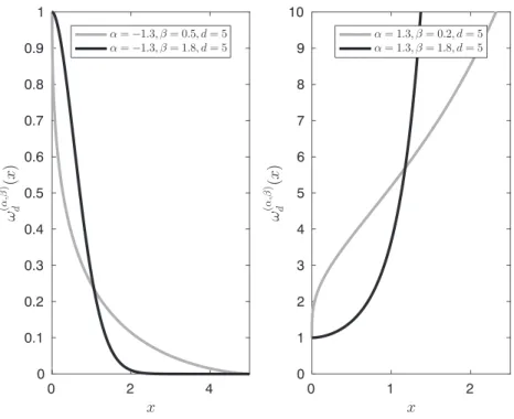
Definition 1. The omega function𝜔^(𝛼,𝛽)_d (x)is given by 𝜔^(𝛼,𝛽)_d (x) =

(d^𝛽+x^𝛽 d^𝛽−x^𝛽

)^𝛼d^𝛽

2 , (3)

where𝛼, 𝛽,d∈R^,𝛽,d > 0,x ∈ (0,d).

Later we will explain why this formula is so useful.

Utilizing the omega function, the density function of the omega probability distribution is given as follows.

Definition 2. The continuous random variable𝜉has an omega probability distribution with the parameters 𝛼, 𝛽,d > 0, if the probability density function𝑓_d^(𝛼,𝛽)(x) of𝜉is given by

𝑓_d^(𝛼,𝛽)(x) =

⎧⎪

⎨⎪

⎩

0, ifx≤0

𝛼𝛽x^𝛽−1_d2𝛽^d−x^2𝛽²^𝛽𝜔^{(−𝛼,𝛽)}_d (x), if 0<x<d

0, ifx≥d,

(4)

where

𝜔⁽⁻_d^𝛼,𝛽⁾(x) =

)^−𝛼d𝛽

2 . (5)

In order to demonstrate that the function𝑓_d^(𝛼,𝛽)(x)given in (4) is in fact a probability density function, we will prove Lemma 1 for which we will utilize the first derivative of the omega function given by Equation 5:

d𝜔⁽⁻_d^𝛼,𝛽⁾(x)

dx = −𝛼𝛽x^𝛽⁻¹ d²^𝛽

d^2𝛽−x^2𝛽𝜔^{(−𝛼,𝛽)}_d (x). (6) Lemma 1. The function 𝑓_d⁽^𝛼,𝛽⁾(x) has the following properties:

1. 𝑓_d^(𝛼,𝛽)(x)≥0for any x∈R^; 2.

∞

∫

−∞

𝑓_d⁽^𝛼,𝛽⁾(x)dx=1.

Proof. The first property of𝑓_d^(𝛼,𝛽)(x)trivially follows.

Utilizing Equation 6, the second property of𝑓_d^(𝛼,𝛽)(x) can be demonstrated as follows:

∞

∫

−∞

𝑓_d^(𝛼,𝛽)(x)dx=

d

∫

0

𝛼𝛽x^𝛽⁻¹ d²^𝛽

d^2𝛽−x^2𝛽𝜔^{(−𝛼,𝛽)}_d (x)dx=

=

[−𝜔^{(−𝛼,𝛽)}_d (x) ]d

0=1.

(7)

Exploiting the above results, it can be shown that the probability distribution function F_d^(𝛼,𝛽)(x) of the random variable𝜉that has an omega probability distribution with

(4)

parameters𝛼, 𝛽,d > 0 is

F⁽^𝛼,𝛽⁾

d (x) =

x

∫

−∞

𝑓_d⁽^𝛼,𝛽⁾(t)dt=

⎧⎪

⎨⎪

⎩

0, ifx≤0

1−𝜔^{(−𝛼,𝛽)}_d (x), if 0<x<d

1, ifx≥d.

(8) It is worth pointing out that the same auxiliary omega function is utilized in the omega probability density and distribution functions. Note that from here on, a probability distribution function always means a cumulative distribution function (CDF). We will show that the omega probability distribution may also be viewed as an alternative to the Weibull probability distribution. For this purpose, first of all, we will discuss the main properties of the omega function.

2.1 Main properties of the omega function

Here, we state the most important properties of the omega function, namely, differentiability, monotonicity, limits, and convexity.

Differentiability. 𝜔^(𝛼,𝛽)_d (x)is a differentiable function in the interval(0,d).

Monotonicity.

• If𝛼 > 0, then𝜔^(𝛼,𝛽)_d (x)is strictly monotonously increasing.

• If𝛼 < 0, then𝜔^(𝛼,𝛽)_d (x)is strictly monotonously decreasing.

• If𝛼 = 0, then𝜔^(𝛼,𝛽)_d (x)has a constant value of 1 in the interval(0,d).

Limits.

xlim→d⁻𝜔⁽_d^𝛼,𝛽⁾(x) =

{∞,if𝛼 >0

0, if𝛼 <0. (9)

Convexity. It can be shown that the shape of function𝜔^(𝛼,𝛽)_d (x)in the interval (0,d)is as follows:

• If

d²^𝛽 < 4( 𝛽²−1)

𝛼²𝛽² , 𝛼≠0, (10)

then𝜔^(𝛼,𝛽)_d (x)is convex when𝛼 > 0 and𝜔^(𝛼,𝛽)_d (x) is concave when𝛼 < 0.

• If

d²^𝛽 ≥ 4( 𝛽²−1)

𝛼²𝛽² , 𝛼≠0, (11)

then we can distinguish the following cases:

-if𝛼 > 0 and 0 < 𝛽 < 1, then𝜔⁽_d^𝛼,𝛽⁾(x)changes its shape from concave to convex atxr;

-if𝛼 > 0 and𝛽 ≥ 1, then𝜔⁽_d^𝛼,𝛽⁾(x)is convex;

-if𝛼 < 0, 0 < 𝛽 ≤ 1, andx_r < d, then𝜔^(𝛼,𝛽)_d (x) changes its shape from convex to concave atxr; -if𝛼 < 0, 0 < 𝛽 ≤ 1, andx_r ≥ d, then𝜔⁽_d^𝛼,𝛽⁾(x) is convex;

-if𝛼 < 0,𝛽 > 1, andx_r < d, then 𝜔⁽_d^𝛼,𝛽⁾(x) changes its shape from concave to convex atxland from convex to concave atx_r; and

-if𝛼 < 0,𝛽 > 1, andxr ≥ d, then 𝜔^(𝛼,𝛽)_d (x) changes its shape from concave to convex atx_l, where

x_l=

(−𝛼𝛽d²^𝛽−√

𝛼²𝛽²d⁴^𝛽−4(𝛽²−1)d²^𝛽 2(𝛽+1)

)_1∕𝛽 , (12)

xr=

(−𝛼𝛽d²^𝛽+√

𝛼²𝛽²d^4𝛽−4(𝛽²−1)d^2𝛽 2(𝛽+1)

)1∕𝛽

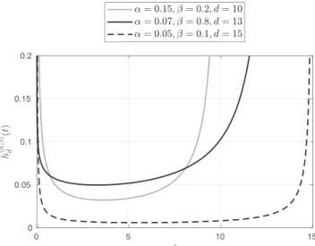
. (13) Figure 1 shows some concrete examples of the omega

function curve.

2.1.1 The generalized exponential differential equation

Now, we introduce the generalized exponential differential equation and show how it is connected with the exponential function𝑓(x) = e^ax^𝛽,(𝛼, 𝛽 ∈ R, 𝛽 > 0)and with the omega function.

Definition 3. We define the generalized exponential differential equation as

d𝑓(x)

dx =𝛼𝛽x^𝛽⁻¹

( d²^𝛽 d^2𝛽−x^2𝛽

)_𝜀

𝑓(x), (14)

where𝜀 ∈ {0,1},𝛼, 𝛽,d ∈ R^,𝛽,d > 0,x ∈ (0,d), f(x) > 0.

Lemma 2. The solutions of the generalized exponential differential equation are

𝑓(x) =

⎧⎪

⎨⎪

⎩

Ce^ax^𝛽, if𝜀=0 C

)^ad𝛽

2 , if𝜀=1, (15)

where C∈R,C>0.

Proof. If𝜀 = 0, then the differential equation in (14) may be written as

d𝑓(x)

dx =𝛼𝛽x^𝛽⁻¹𝑓(x). (16) Separating the variables in (16) and integrating both sides lead to

∫ 1

𝑓(x)d𝑓(x) =

∫ 𝛼𝛽x^𝛽−1dx, (17)

(5)

FIGURE 1 Examples of omega function curves

ln|𝑓(x)|=𝛼x^𝛽+lnC, (18) whereC > 0. Utilizing the fact thatf(x) > 0, the last equation may be written as

𝑓(x) =Ce^𝛼x^𝛽. (19) If 𝜀 = 1, then the differential equation in (14) becomes

d𝑓(x)

dx =𝛼𝛽x^𝛽−1 d²^𝛽

d^2𝛽−x^2𝛽𝑓(x). (20) Exploiting the fact that

1

d²^𝛽−x²^𝛽 = 1 2d^𝛽

( 1

d^𝛽+x^𝛽 + 1 d^𝛽−x^𝛽

), (21)

separating the variables in (20), and integrating both sides give

∫ 1

𝑓(x)d𝑓(x) =𝛼𝛽d^𝛽 2

(

∫ x^𝛽−1 d^𝛽+x^𝛽dx+

∫ x^𝛽−1 d^𝛽−x^𝛽dx

) , (22) ln|𝑓(x)|= 𝛼d^𝛽

2

(ln|d^𝛽+x^𝛽|−ln|d^𝛽−x^𝛽|)

+lnC, (23) whereC > 0. Sincef(x) > 0 andx ∈ (0,d), the last equation may be written as

𝑓(x) =C

)^𝛼^d𝛽

2 . (24)

2.1.2 Connections between

the exponential and omega functions

Lemma 2 suggests that there is an important connection between the exponential function 𝑓(x) = e^ax^𝛽 and the omega function. Namely, the solution of the generalized exponential differential equation for 𝜀 = 0 and C = 1 is simply the exponential function 𝑓(x) = e^𝛼^x^𝛽, while the solution of (14) for 𝜀 = 1, C = 1 is the omega function. Furthermore, ifdis much greater thanx, then

d²^𝛽

d²^𝛽−x²^𝛽 ≈1, (25) and the generalized exponential differential equation for 𝜀 = 1 becomes the following approximate equation:

d𝑓(x)

dx ≈𝛼𝛽x^𝛽⁻¹𝑓(x), (26) which is nearly the generalized exponential differential equation with𝜀 = 0, the solution of which is the exponential function𝑓(x) =e^𝛼^x^𝛽. The following theorem provides the theoretical basis for this result.

Theorem 1. For any x ∈ (0,d)and𝛽 > 0,

d→∞lim𝜔^(𝛼,𝛽)_d (x) =e^𝛼^x^𝛽. (27)

Proof. Letxhave a fixed value, where againx ∈ (0,d).

(6)

d→∞lim𝜔^(𝛼,𝛽)_d (x) = lim

d→∞

)^𝛼d^𝛽

2

= lim

d→∞

((d^𝛽−x^𝛽+2x^𝛽 d^𝛽−x^𝛽

)d^𝛽)^𝛼

2

=

= lim

d→∞

((

1+ 2x^𝛽 d^𝛽−x^𝛽

)d^𝛽)^𝛼

2

.

(28)

Sincexis fixed, ifd → ∞, thenΔ = d^𝛽 − x^𝛽 → ∞ and so the previous calculation can be continued as follows:

dlim→∞

((

1+ 2x^𝛽 d^𝛽−x^𝛽

)d^𝛽)^𝛼

2

= lim

Δ→∞

((

1+ 2x^𝛽 Δ

)Δ+x^𝛽)^𝛼

2

=

= (

Δ→∞lim (

1+ 2x^𝛽 Δ

)Δ Δ→∞lim

( 1+ 2x^𝛽

Δ )x^𝛽)^𝛼₂

= (

e^2x^𝛽 )^𝛼

2 ·1^a² =e^𝛼x^𝛽.

(29) On the basis of Theorem 1, it can be stated that the asymptotic omega function is just the exponential function 𝑓(x) =e^𝛼^x^𝛽. Actually, ifx ≪ d, then𝜔⁽_d^𝛼,𝛽⁾(x) ≈e^𝛼^x^𝛽; that is, ifdis sufficiently large, then the omega function suitably approximates the exponential function𝑓(x) =e^𝛼^x^𝛽.

2.2 An approximation to the Weibull probability distribution

If the random variable 𝜂 has a two-parameter Weibull probability distribution with the parameters𝛼, 𝛽 > 0, then the probability density functionf^(𝛼,𝛽)(x)of𝜂is given by

𝑓^(𝛼,𝛽)(x) =

{0, ifx≤0

𝛼𝛽x^𝛽⁻¹e⁻^𝛼^x^𝛽, ifx>0. (30) The next lemma tells us how the omega probability distribution is connected with the Weibull probability distribution.

Lemma 3. For any x∈R^and𝛼, 𝛽 > 0, if d→∞, then

𝑓_d^(𝛼,𝛽)(x)→𝑓^(𝛼,𝛽)(x). (31)

Proof. Letx∈Rbe fixed. We will now distinguish the following two cases.

• Ifx ≤ 0 orx ≥ d, then𝑓_d^(𝛼,𝛽)(x) = 𝑓^(𝛼,𝛽)(x) = 0 holds by definition.

• Ifx ∈ (0,d),d > 0, then 𝑓_d^(𝛼,𝛽)(x) =𝛼𝛽x^𝛽−1 d^2𝛽

d²^𝛽−x²^𝛽𝜔^{(−𝛼,𝛽)}_d (x). (32) Ifd→∞, then

d²^𝛽

d²^𝛽−x²^𝛽 →1, (33)

FIGURE 2 Plots of Weibull and omega probability density functions

(7)

and following Theorem 1,

𝜔^{(−𝛼,𝛽)}_d (x)→e⁻^𝛼^x^𝛽. (34) That is, ifd→∞, then

𝑓_d^(𝛼,𝛽)(x)→𝛼𝛽x^𝛽⁻¹e⁻^𝛼^x^𝛽 =𝑓⁽^𝛼,𝛽⁾(x). (35)

Figure 2 shows some examples of how the omega probability density function can approximate the Weibull probability density function. In each subplot of Figure 2, the left-hand side scale is associated with functions f^(𝛼,𝛽)(x) (gray line) and 𝑓_d⁽^𝛼,𝛽⁾(x) (dashed black line), while the right-hand side scale is connected with the difference func- tion𝑓⁽^𝛼,𝛽⁾(x) −𝑓_d⁽^𝛼,𝛽⁾(x)(thin black line). Table 1 shows the maximum and the mean of absolute differences between f⁽^𝛼^,^𝛽⁾(x)and𝑓_d⁽^𝛼,𝛽⁾(x)for the plots shown in Figure 2. We can see that, in line with Lemma 3, the goodness of approximation improves asdincreases.

If the random variable𝜂 has a two-parameter Weibull probability distribution with the parameters𝛼, 𝛽 > 0, then the probability distribution functionF⁽^𝛼^,^𝛽⁾(x)of𝜂is given by

F^(𝛼,𝛽)(x) =

{0, ifx≤0

1−e^−ax^𝛽,ifx>0. (36) Theorem 2. For any x ∈ R^,𝛼, 𝛽,d > 0, if the ran- dom variable𝜉 has an omega probability distribution with the parameters𝛼, 𝛽,d and the𝜂random variable has a Weibull probability distribution with parameters 𝛼, 𝛽, then

d→∞limP(𝜉 <x) =P(𝜂 <x). (37) Proof. SinceF_d^(𝛼,𝛽)(x) =P(𝜉 < x)andF^(𝛼,𝛽)(x) =P(𝜂 <

x)for anyx∈ R, using the definitions ofF⁽^𝛼,𝛽⁾

d (x)and F^(𝛼,𝛽)(x), this theorem follows from Theorem 1.

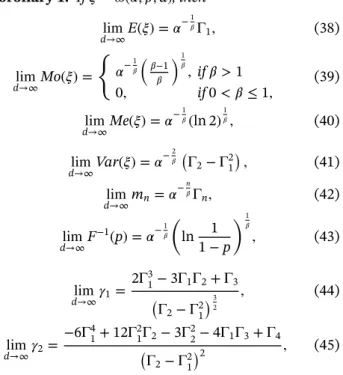
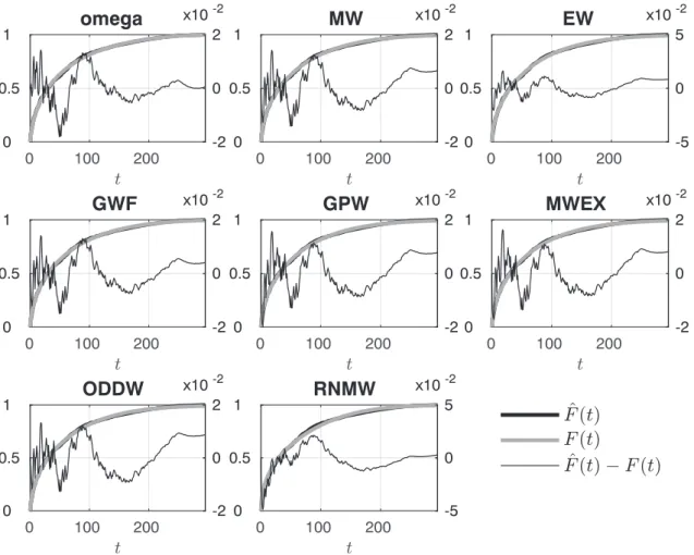
Some examples of Weibull probability distribution functions and their approximations by the omega probability distribution functions are shown in Figure 3. Similar to Figure 2, in each subplot of Figure 3, the left-hand side scale is associated with functionsF^(𝛼,𝛽)(x)(gray line) and F_d^(𝛼,𝛽)(x)(dashed black line), while the right-hand side scale

TABLE 1 Errors of approximations to Weibull probability density functions

d max

x∈(0,d)|||𝑓^(𝛼,𝛽)(x) −𝑓_d⁽^𝛼,𝛽⁾(x)||| ¹^d

d

∫

0|||𝑓^(𝛼,𝛽)(x) −𝑓_d⁽^𝛼,𝛽⁾(x)|||dx

5 1.5498e-02 7.0973e-03

10 1.4812e-03 5.6295e-04

15 4.3621e-04 1.1082e-04

20 1.8376e-04 3.5031e-05

is connected with the difference functionF^(𝛼,𝛽)(x)−F^(𝛼,𝛽)

d (x) (thin black line). Table 2 shows the maximum and the mean of absolute differences betweenF^(𝛼,𝛽)(x)andF⁽^𝛼,𝛽⁾

d (x) for the examples in Figure 3. We can see that the goodness of approximation improves asdincreases.

On the basis of Theorem 2, it can be stated that the asymptotic omega probability distribution is just the Weibull probability distribution. Thus, in practical applications, the Weibull probability distribution with parameters 𝛼, 𝛽 > 0 can be substituted by the omega probability distribution that has the parameters𝛼, 𝛽,d > 0, ifx ≪ d.

It is worth mentioning that while the Weibull probability distribution function is a transcendental function, the omega probability distribution function is a power function. This means that from a computational point of view, the omega probability distribution function is more con- venient than the Weibull probability distribution function.

This feature of the omega probability distribution further enhances its applicability in problems where computation time is a critical factor.

From here on, we will use the notations𝜉 ∼ 𝜔(𝛼, 𝛽,d) and𝜂 ∼ W(𝛼, 𝛽)to indicate that𝜉 has an omega probability distribution with the parameters𝛼, 𝛽,d > 0 and𝜂 has a Weibull probability distribution with the parameters 𝛼, 𝛽 > 0, respectively.

2.3 Asymptotic properties of the omega probability distribution

The next corollary summarizes the main asymptotic characteristics of the random variable that has an omega probability distribution.

Corollary 1. If𝜉∼𝜔(𝛼, 𝛽,d), then

d→∞limE(𝜉) =𝛼⁻¹^𝛽Γ1, (38)

d→∞limMo(𝜉) = {

𝛼⁻^𝛽¹(

𝛽−1 𝛽

)¹

𝛽, if𝛽 >1

0, if0< 𝛽≤1, (39)

d→∞limMe(𝜉) =𝛼⁻¹^𝛽(ln 2)

1

𝛽, (40)

dlim→∞Var(𝜉) =𝛼⁻^𝛽²(

Γ₂− Γ²₁)

, (41)

dlim→∞m_n=𝛼⁻ⁿ^𝛽Γn, (42)

d→∞limF⁻¹(p) =𝛼⁻¹^𝛽 (

ln 1 1−p

)¹

𝛽, (43)

dlim→∞𝛾1= 2Γ³₁−3Γ1Γ2+ Γ3

(Γ2− Γ²₁)³

2

, (44)

d→∞lim𝛾2= −6Γ⁴₁+12Γ²₁Γ2−3Γ²₂−4Γ1Γ3+ Γ4

(Γ2− Γ²₁)2 , (45)

(8)

FIGURE 3 Examples of Weibull and omega probability distribution functions

TABLE 2 Errors of approximations to Weibull probability distribution functions

d max

x∈(0,d)|||F⁽^𝛼,𝛽⁾(x) −F_d⁽^𝛼,𝛽⁾(x)||| ¹^d

d

∫

0

|||F⁽^𝛼,𝛽⁾(x) −F⁽_d^𝛼,𝛽⁾(x)|||dx

5 2.3459e-02 1.1677e-02

10 2.8164e-03 9.9133e-04

15 8.3117e-04 2.0060e-04

20 3.5031e-04 6.3862e-05

where E(𝜉), Mo(𝜉), Me(𝜉), Var(𝜉), m_n, F⁻¹(p),𝛾1, and 𝛾2 are the mean, mode, median, variance, nth raw moment, quantile function, skewness, and kurtosis excess of the random variable𝜉, respectively, and

Γi= Γ (

1+ i 𝛽

)

. (46)

Here, 0 < p < 1, and 𝛤 denotes Euler's gamma function.

Proof. On the basis of Theorem 2, if d → ∞, then P(𝜉 < x) = P(𝜂 < x), where the random vari- able𝜂has a Weibull distribution with the parameters 𝛼, 𝛽 > 0. The corollary can be proven by utilizing this result and the characteristics of the Weibull probability distribution.

It should be added that the analytic calculations of the main characteristics of the omega probability distribu-

tion including the mean, mode, median, variance, nth raw moment, quantile function, skewness, and kurtosis excess lead to complicated integrals and formulas that are difficult to deal with. At the same time, in practical reliability engineering applications, the omega probability distribution is typically deployed with a value of parameter d that is sufficiently large to utilize the result of Theorem 2 and Corollary 1, which allow us to substitute the above-mentioned characteristics of the probability distribution with their asymptotic values. For example, if we have weekly failure data for a year, then the time horizon of the analyses is 52 weeks, and sod ≥ 52. In such a case, the asymptotic values of the characteristics can be utilized instead of their exact values.

2.4 Interpretation of parameters

The omega probability distribution has three parameters, namely, the parameters𝛼,𝛽, andd, which are all positive.

On the basis of the definition of the probability density function 𝑓_d⁽^𝛼,𝛽⁾(x) of the omega probability distribution, the parameterdspecifies the support of𝑓_d^(𝛼,𝛽)(x); that is, 𝑓_d^(𝛼,𝛽)(x)is positive only if x ∈ (0,d). By Theorem 2, we have demonstrated that ifd → ∞, then the omega probability distribution is identical with the two-parameter Weibull probability distribution given in (2). This result also indicates that if the value of parameterdis sufficiently large, then the role of the parameters𝛼and𝛽of the omega probability distribution is very similar to those of the cor-

(9)

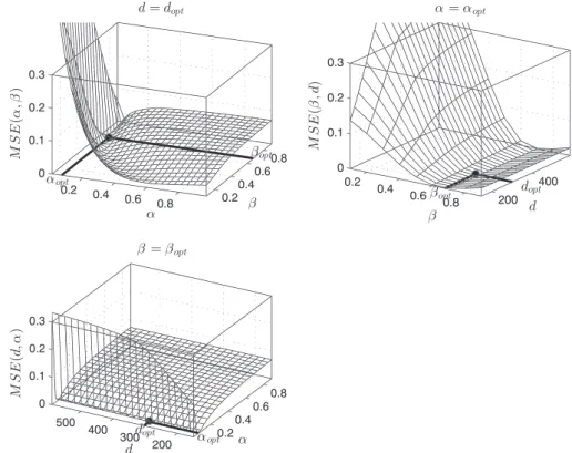
FIGURE 4 Interpretation of parameters

responding𝛼and𝛽parameters of the Weibull probability distribution. Note that even ford ≥ 5, the omega probability distribution approximates the Weibull probability distribution quite well (see Figures 2 and 3).

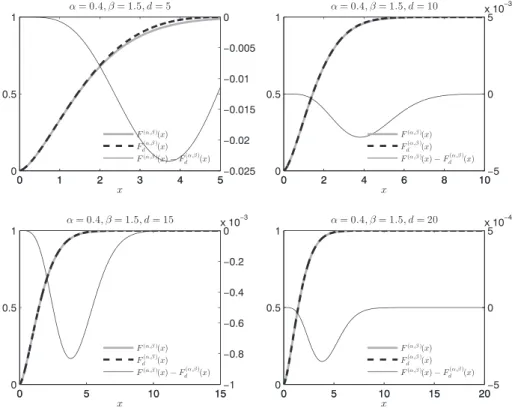
Figure 4 shows how the parameters𝛼and𝛽 affect the characteristics of the omega probability density function.

The parameter𝛼may be viewed as the scale parameter of the distribution; that is, the greater the value of𝛼is, the greater the maximum value of the density function is. The parameter𝛽affects the shape of the density function in the following way:

• If 0 < 𝛽 < 1, then lim_x→0⁺𝑓_d^(𝛼,𝛽)(x) = ∞and𝑓_d^(𝛼,𝛽)(x)is strictly monotonously decreasing forx > 0.

• If 𝛽 = 1, then 𝑓_d^(𝛼,𝛽)(0) = 𝛼 and 𝑓_d^(𝛼,𝛽)(x) is strictly monotonously decreasing forx > 0.

• If 𝛽 > 1, then 𝑓_d^(𝛼,𝛽)(x) has its maximum at x ≈ 𝛼^−1/𝛽((𝛽 − 1)∕𝛽)^1/𝛽.

It is also worth mentioning that the asymptotic skewness and the asymptotic kurtosis excess of the omega probability distribution given by (44) and (45), respectively, depend only on the parameter𝛽. Hence, the parameter𝛽may be viewed as the shape parameter of the omega probability distribution.

2.5 Statistical estimation of parameters

Here, we will discuss two methods for the parameter estimation of the omega distribution. Firstly, we will provide the log-likelihood function and propose a method to maxi- mize it. Secondly, we will discuss how the parameters of the

omega distribution can be estimated by fitting its CDF to an empirical CDF. Here, we assume that the random vari- able𝜏represents the time-to-first-failure of a component or system and𝜏has an omega probability distribution with the parameters𝛼, 𝛽,d > 0. It should be highlighted that the above-mentioned two methods utilize different data set types. In the case of maximum likelihood estimation, we assume that independent and identically distributed t1,t2,…,tnobservations are available on the random variable 𝜏. However, in many cases of practical reliability engineering, the exactt1,t2,…,tntime-to-first-failure data are not available, rather we have frequency data indicating the number of components or systems that have failed in given time periods. In such cases, the empirical CDF of𝜏 can be directly produced, and the second method, which estimates the parameters by fitting the omega CDF to the empirical CDF of𝜏, can be applied.

2.5.1 Maximum likelihood estimation

Lett1,t2,…,tnbe independent and identically distributed observations on the random variable𝜏and𝜏 ∼𝜔(𝛼, 𝛽,d).

Utilizing the definition of the omega probability density function 𝑓_d⁽^𝛼,𝛽⁾(x) given by (4), the likelihood function L(𝛼, 𝛽,d)is

L(𝛼, 𝛽,d) =

∏n

i=1

𝑓_d^(𝛼,𝛽)(ti) =

=𝛼ⁿ𝛽ⁿ

∏n

i=1

⎛⎜

⎜⎜

⎝

t^𝛽−1_i d^2𝛽 d^2𝛽−t²_i^𝛽

(d^𝛽+t^𝛽_i d^𝛽−t^𝛽_i

)^−𝛼^d𝛽

2 ⎞

⎟⎟

⎟⎠ .

(47)

(10)

The log-likelihood functionl(𝛼, 𝛽,d) =ln(L(𝛼, 𝛽,d))is l(𝛼, 𝛽,d) =nln𝛼+nln𝛽+ (𝛽−1)

∑n

i=1

lnt_i+

+

∑n

i=1

ln d²^𝛽

d^2𝛽−t_i^2𝛽 −𝛼d^𝛽 2

∑n

i=1

lnd^𝛽+t_i^𝛽 d^𝛽−t_i^𝛽.

(48) Notice that according to Definition 2, the parameterd specifies the support of𝑓_d⁽^𝛼,𝛽⁾(x); that is,𝑓_d⁽^𝛼,𝛽⁾(x)is positive only ifx ∈ (0,d). It means that the value of parame- ter d needs to satisfy the condition d > max_i=1,…_,n(t_i).

So the maximum likelihood estimations of the parame- ters𝛼,𝛽, anddcan be obtained by solving the following minimization problem:

−l(𝛼, 𝛽,d)→min 𝛼, 𝛽,d>0 d> max

i=1,…,n(t_i).

(49)

There is no closed form solution for this minimization problem; it can be solved by utilizing a global optimiza- tion method. We propose the application of the so-called GLOBAL method, which is a stochastic global optimiza- tion procedure introduced by Csendes et al.⁴⁵^,⁴⁶

It is worth mentioning that there is an interesting connection between the log-likelihood functions of the Weibull and omega probability distributions. On the one hand, the log-likelihood function of the Weibull probability distribution given by the probability density function in (2) is

l(𝛼, 𝛽) =nln𝛼+nln𝛽+ (𝛽−1)

∑n

i=1

lnt_i−𝛼

∑n

i=1

t_i^𝛽. (50) On the other hand,

dlim→∞

( _n

∑

i=1

ln d²^𝛽 d²^𝛽−t²_i^𝛽

)

=0, (51)

and on the basis of Theorem 1,

d→∞lim (𝛼d^𝛽

2

∑n

i=1

lnd^𝛽+t^𝛽_i d^𝛽−t^𝛽_i

)

=𝛼

∑n

i=1

t_i^𝛽. (52) Hence, ifd → ∞, then the log-likelihood function of the omega probability distribution in (48) is identical with the log-likelihood function of the Weibull probability distribution given by (50).

2.5.2 Fitting the cumulative probability distribution function

LetN(t)denotes the number of components or systems that have survived up to timetfrom the number of components or systemsN(0)that were initially put into operation. Let Δt denotes the length of a time period, and lett = iΔt,

wherei = 0,1,…,nandΔt > 0. IfΔt = 1, then the N(t) − N(t + Δt)difference, which represents the number of components or systems that fail in the time interval (t,t + Δt], isN(i) − N(i + 1), wherei = 0,1,…,n − 1.

For example, ifΔt = 1 week, then the differenceN(3) − N(4)represents the number of components or systems that failed on the fourth week. As noted before, there are cases in practice, when the exactt1,t2,…,tntime-to-first-failure data are not available, rather frequency data are available indicating the number of components or systems that have failed in given time periods. In such cases, when the N(0),N(1),…,N(n)data are available, the empirical CDF F(t)̂ of the time-to-first-failure random variable 𝜏can be computed as

F(i) =̂ 1− N(i)

N(0), (53)

where i = 0,1,…,n. Next, the parameters𝛼,𝛽, andd of the omega probability distribution can be identified by fitting the omega CDFF^(𝛼,𝛽)_d (t)to the empirical CDFF(t).̂ For this purpose, we need to minimize the following sum of squares:

S(𝛼, 𝛽,d) =

∑n

i=1

( F⁽^𝛼,𝛽⁾

d (i) −F(i)̂ )2

, (54)

with the constraints 𝛼, 𝛽,d > 0. This minimization problem can be solved by utilizing the GLOBAL method that we referenced in Section 2.5.1. In our demonstrative example (Section 3.2), we will show how the CDF fitting method can be applied in practice.

3 N OV E L M O D E L S O F

BAT H T U B- S H A P E D H A Z A R D C U RV E S

Now, potential applications of the omega probability distribution for failure rate function modeling will be discussed.

We will demonstrate that the so-called omega HF can be viewed as a suitable model of bathtub-shaped failure rate functions.

Here again, let the random variable𝜏 be the time-to- first-failure of a component or system. It is well known that a typical HF curve of a component or a system is bathtub shaped; that is, it can be divided into three distinct phases called the infant mortality period, useful life, and wear-out period. It is also typical that the probability distribution of 𝜏 is different in the three characteristic phases of the bathtub-shaped HF. If𝜏has a Weibull probability distribution with the parameters𝛼, 𝛽 > 0, then the HFh^(𝛼,𝛽)(t)of 𝜏, which we call the Weibull HF, is

h^(𝛼,𝛽)(t) =𝛼𝛽t^𝛽−1. (55)

We can see from (55) a notable property of the HFh⁽^𝛼^,^𝛽⁾(t).

Namely,

(11)

• if 0 < 𝛽 < 0, thenh^(𝛼,𝛽)(t)is decreasing,

• if𝛽 = 1, thenh⁽^𝛼^,^𝛽⁾(t)is constant with the value of𝛼𝛽,

• if𝛽 > 1, thenh^(𝛼,𝛽)(t)is increasing

with respect to time. This property of the Weibull HF indicates that each of the three characteristic phases of a bathtub-shaped hazard curve can be described by an appropriate Weibull HF. That is, three Weibull HFs, a decreasing, a constant, and an increasing, connected to each other can exhibit a bathtub-shaped hazard curve.

This universality of the Weibull probability distribution makes it suitable for modeling the probability distribution of time-to-first-failure random variable in a wide range of reliability analyses.

3.1 The omega hazard function

Now, let us assume that𝜏has an omega probability distribution with the parameters𝛼, 𝛽,d > 0. In this case, the HFh^(𝛼,𝛽)_d (t)of𝜏, which we will call the omega HF, is

h⁽^𝛼,𝛽⁾

d (t) = 𝑓_d^(𝛼,𝛽)(t)

1−F_d^(𝛼,𝛽)(t) = 𝛼𝛽t^𝛽−1_d2^d𝛽−t^2𝛽²^𝛽𝜔^{(−𝛼,𝛽)}_d (t) 𝜔^{(−𝛼,𝛽)}_d (t) =

=𝛼𝛽t^𝛽−1 d²^𝛽 d^2𝛽−t^2𝛽,

(56)

if 0 < t < d. Utilizing (55) and (56), the omega HFh⁽^𝛼,𝛽⁾

d (t) may be written as

h^(𝛼,𝛽)_d (t) =h⁽^𝛼,𝛽⁾(t)g^(𝛽)_d (t), (57)

where

g^(𝛽)_d (t) = d²^𝛽

d^2𝛽−t^2𝛽, (58) and𝛼, 𝛽,d > 0,t ∈ (0,d). That is, the omega HF may be viewed as the Weibull HF multiplied by the corrector functiong^(𝛽)

d (t).

The omega HFh^(𝛼,𝛽)_d (t)has some important properties that make it suitable for modeling bathtub-shaped failure rate curves.

3.1.1 Piecewise modeling

The following lemma states a key property of the omega HF h⁽^𝛼,𝛽⁾

d (t). It allows us to utilize the omega HF as an alternative to the Weibull HF.

Lemma 4. For any t ∈ (0,d), if d → ∞, then h^(𝛼,𝛽)_d (t)→h^(𝛼,𝛽)(t), where𝛼, 𝛽,d > 0.

Proof. Ift ∈ (0,d)is fixed andd→∞, theng^(𝛽)_d (t)→1 and so

h^(𝛼,𝛽)

d (t) =h^(𝛼,𝛽)(t)g^(𝛽)

d (t)→h^(𝛼,𝛽)(t). (59)

The practical implication of this result is as follows.

Since the Weibull HF can be utilized as a model for each phase of a bathtub-shaped failure rate curve andh^(𝛼,𝛽)_d (t) ≈ h⁽^𝛼,𝛽⁾(t), iftis small compared withd, the omega HF can also model each phase of the same bathtub-shaped failure rate curve, ifdis sufficiently large. That is, the omega

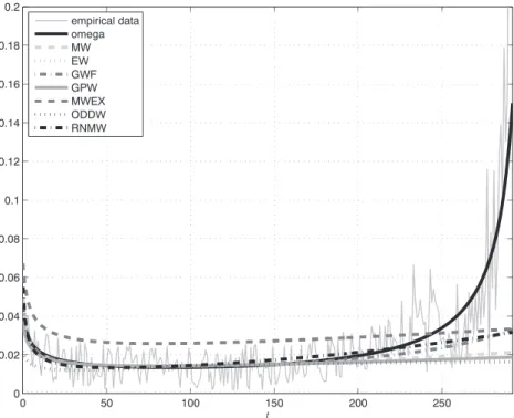
FIGURE 5 Plots of Weibull and omega hazard function curves