Magnetically with

C H A P T E R 6

Systems with Two Groups of Magnetically Equivalent Nuclei

T h e stationary hamiltonian operator for a spin system composed of two groups of magnetically equivalent s p i n - \ nuclei is given by (1-6)

& = —{^A^Az + OJBIBz + J lA ' IB}

where / = /A B = JBA , and where the spin-spin interactions within each group have been omitted (cf. Section 4, Chapter 5). This hamiltonian admits three constants of the motion: IA 2 , IB 2, andlz = I^Az -f- IBz . An initial basis for the analysis of the eigenvalue problem is provided by the set of all product kets {| IA , ηι^Α}\ I^B , m^B)}.

Before proceeding with the study of particular systems, it will be convenient to adopt certain conventions concerning the relative mag- nitudes of ω^Α and ω^Β , the sign of / , and the classification of transitions.

(1) For systems with nA > n^B , all theoretical spectra will be calculated on the assumption ωΑ > ω^Β , so that the internal chemical shift

δ = ωΑ — α>Β

is a positive quantity. Graphical representations of theoretical spectra with nA > n^B will be drawn with the frequency origin at ωΒ . By reflecting these graphs in the line ω = ωΒ -f- ^ δ — ^(ωΑ + ωΒ), one obtains the graphs for the case where ωΑ < ωΒ . It will be shown in Section 4 that when n^A = n^B , the spectrum is symmetrical with respect to a frequency origin at \(ωΑ + ω^Β).

(2) Since the steady-state spectrum of any two-group system does not depend upon the sign of / , it will be arbitrarily assumed that / > 0.

(3) All theoretical calculations will use angular frequency units for Larmor frequencies and coupling constants. T h e theoretical expressions

1 8 7

188 6. SYSTEMS WITH MAGNETICALLY EQUIVALENT NUCLEI

A T r a n s i t i o n s Β T r a n s i t i o n s M T r a n s i t i o n

(1, I) - ( 0 , i) (L, i ) - d , -I) (1, - « - ( - 1 , «

(1, - 4 ) - ( 0 , -i) (0, « - ( 0 , - è) (0, I ) - ( - I . I ) ( - 1 , I ) - ( - L , - I ) (0, - J ) - ( - 1 , - è )

This method of classifying transitions, which may also be used to describe the transitions of a system composed of an arbitrary number of magnetically equivalent groups, is merely a convenient bookkeeping method. When / Φ 0, an allowed transition involves two linear com- for the relative signal intensities depend only on the ratio of the param- eters J and δ, so that these quantities do not depend upon the choice of units. T h e expressions for the resonance frequencies may be converted to linear frequency units by dividing by 2π> but inasmuch as there is an arbitrary scale factor in any experimental spectrum, all theoretical expressions for the resonance frequencies may be applied to practical computations as though they were computed in linear units. However, notational consistency will be maintained by writing 8/2π and / / 2 7 r for the chemical shift and spin-spin coupling constant in linear frequency units.

(4) Transitions will be classified according to the limiting values of their resonance frequencies when / — • ( ) . T h e limiting resonance frequencies are of the form — (O>A AmA -f- A>B AmB)y where AmA -\- AmB = Am = — 1 .

A transition whose resonance frequency approaches a>G as / —• 0 is said to be a transition in group G. Evidently, a transition in group G is such that AmG = — 1, while AmG> = 0, G, G' = A, B (G Φ G').

A transition whose resonance frequency approaches a linear combina- tion of Larmor frequencies is said to be a mixed transition. For a mixed transition, AmA Φ 0, AmB Φ 0, subject, of course, to the general restriction Am = AmA + AmB = — 1 .

T o illustrate these definitions, consider the irreducible A1B1/2 system.

T h e A, B, and M transitions are determined by enumerating all possible changes (mA , m^B) —> (m^Ay raB'), consistent with IA = 1, IB — ^ , and Am^A + Am^B = — 1. A simple calculation shows that there are four transitions in group A, three in group B, and one mixed transition (see accompanying tabulation). T h e limiting frequencies of the A, B, and M transitions are ωΑ, CUB , and 2ωΑ — ω^Β , respectively.

1. T H E AB S Y S T E M 189 binations of product kets. For convenience, one speaks of the transition in terms of the product kets to which these linear combinations reduce as / - * 0 .

1. The AB System A. Diagonalization of the Hamiltonian Matrix

T h e simplest two-group system is the irreducible AB system (AB = A1/2B1/2) . T h e only nontrivial constant of the motion in a steady ζ field is Iz, so that a suitable initial basis is provided by the product kets

I + + > , I + — >, I — + > , I >, whose Iz eigenvalues are 1, 0, 0, — 1, respectively. Operating on the elements of this basis with yields

# I + + > = -

\])\

# I + - > = -

i O I + - > -

I - + > ,

I - + > =

i / ) l - + > -

I + - > ,

* \ — > = £ ( " A + ω^Β -

\])\

vectors of (1.2) and (1.3) show that the two eigenvectors of Jf7 with m = 0, to be denoted | 0; 1> and | 0; 2>, are linear combinations of I [-> and I H ) . Note that the hamiltonian matrix for the AB system could have been written down immediately by replacing all spin operators in the hamiltonian with the appropriate Kronecker products given in Table 4.1.

T h e eigenvalues and eigenvectors of 3 ^ corresponding to m = 0 are obtained by diagonalizing the 2 x 2 submatrix of defined by (1.2) and (1.3):

* < » - ; ( * ' - - / I R A

T h e eigenvalues of this matrix, obtained by solving det[Jf (0) are

ßI(0) = ^{IIIJ +} #1/2.-1/2), Ω2(0) = I ( I / — #1/2,-1/2)»

where1

*!/..-!/. = (δ² + ^J2)'12- (1.7)

- Ω1] = 0, (1.6)

1 T h e significance of t h e n o t a t i o n a l a b b r e v i a t i o n s i n t r o d u c e d h e r e a n d in t h e following section will b e indicated in Section 3.

190 6. S Y S T E M S W I T H M A G N E T I C A L L Y E Q U I V A L E N T N U C L E I

(*'-"/ u t i ® - ™ ®

2

From this matrix equation one obtains two linear equations for a$ and bj . These equations are not independent, but either equation can be com- bined with the normalization condition to determine | 0; 1> and | 0; 2>.

The calculation is straightforward and yields

| 0 ; 1 >

=TTT7W

(1.10) 1

where

1 0 î 2> = (1 + Q\^I% l / 2) î 7 ï ( g i / 2. - i/ 2 ! - + > + ! + - » >

ö l/ 2, - l/ 2 — Si \ j ' ( I ' l l )

° ~ Γ ^ 1/ 2, - 1/ 2

and where the phases of uj and bj have been chosen so as to make these quantities real. The eigenvalues and eigenvectors of the AB system are collected in Table 6.1.

T A B L E 6.1

EIGENVALUES A N D EIGENVECTORS FOR THE A B S Y S T E M

Eigenvector Eigenvalue

1 + + > — è ( ^ A + ω Β ) —

U

1

"(I - + > - 0 1/ 2. - 1/ 2 1 + ->}

(1 f- ^{Q2 )1 /2}

^ 1/ 2, - 1/ 2 '

"(I - + > - 0 1/ 2. - 1/ 2 1 + ->}

1

- { 0 1/ 2. - 1/ 2 1 - + > + 1 +

ι - - >

->} ^{\{\J - Ä1 / 2. _1 / 8)}

ϋ

Α

U

(i -' ^ 1 / 2 , - 1 / 2 '

- { 0 1/ 2. - 1/ 2 1 - + > + 1 +

ι - - >

->} ^{\{\J - Ä1 / 2. _1 / 8)}

ϋ

Α

U

T h e eigenvectors of

3tf(0)

j

I - + >

1 . T H E AB S Y S T E M 191

Β. Spectra of AB Systems

T h e spectrum of an AB system is generated by transitions | j} —>- | k}

satisfying Am = - 1 . T h e resonance frequencies are computed by the Bohr frequency rule, and the corresponding relative intensities are propor- tional to the absolute squares of (k\ I~ \j} = <A| I^A~ \j} + (k\ I^B~ Ij)- Operating on the stationary eigenvectors with I~y one obtains, after some elementary algebra,

/-!++> = I+-> + ! - +>

=

- ϊΗ—) ^{I ° ; Ο}

I

I

— ) I >,

X ^ l/ 2, - l/ 27

/ - | 0 ; 2 > = (l I >,

V ^ 1/ 2, - 1/ 27

7 - | > = 0 .

It follows that there are exactly four transitions satisfying Am = — 1 :

A. | l+ + > - | 0 ; l > , B. II + + > - > | 0 ; 2 > , 0 ; 2 > — | >, ' l | 0 ; l > — | >.

T h e A transitions correspond, in the limit / —> 0, to transitions for which AmA = — 1 and ΔτηΒ = 0; the Β transitions correspond to ΔτηΑ = 0 and J m^B = —1 . T h e relative intensities of these transitions are given by

|<0; 1 11-

|. + +>|* = |< I

| < 0 ; 2 | / - | + + > | » = |< | / - | 0 ; 2 > | » = 1 +

^ 1/ 2, - 1/ 2

/

^ 1/ 2, - 1/ 2

T h e corresponding resonance frequencies are obtained by computing the differences of the appropriate energy eigenvalues given in Table 6.1.

T h e complete spectrum is given in Table 6.2, where, according to the conventions adopted above, the resonance frequencies2 are in the order A i > A² > B² > B¹ .

2 H e r e , a n d s u b s e q u e n t l y , t h e s y m b o l Gt will b e u s e d t o d e n o t e t h e ith t r a n s i t i o n in g r o u p G a n d t h e c o r r e s p o n d i n g r e s o n a n c e f r e q u e n c y . T h e intensity of G* will b e d e n o t e d I n t Gi . Similarly, Μ,· a n d I n t Mt- d e n o t e t h e f r e q u e n c y a n d intensity of t h e m i x e d t r a n s i - tion Μ , · .

192 6. S Y S T E M S W I T H M A G N E T I C A L L Y E Q U I V A L E N T N U C L E I

B2 : I + + > - > I + - > 1 + — ^ ί ( ωΑ + COB + / - # 1 / 2 . - 1 / 2 )

• " 1 / 2 . - 1 / 2

a T r a n s i t i o n in t h e limit / - > 0.

From Table 6.2 it is evident that the AB spectrum is symmetrical with respect to the mean resonance frequency ^ ( ωΑ + ωΒ), and that the following intensity relations hold:

Int A¹ = Int B^t, Int A2 = Int B2, Int A¹ < Int A2, Int Ax + Int A2 = 2,

Int Ax + Int A2 + Int B1 + Int B2 = 4.

T h e last equation also follows from the general formula for nA + nB ··· = Ν spin-^ nuclei,

I n t A^{n A}B^{n ß}C^{n c}- = 2^-W, (1.12)

or the general formula for the intensity of an irreducible component system

I n t A/ AB/ BC/ c ... = \H(2IG + 1) j ^ /G( /G + 1)1 (1.13)

G ' G '

(cf. Section 4.F, Chapter 5). For the irreducible Α^{/ Α}Β^{/ β} system, (1.13) reduces to

Int A/AΒ/ B = f ( 2 /A + 1)(2/B + 1 ) { /A( /A + 1) + h{h + 1)}· (1.14) If 7^A = I^B = J , (1.14) yields Int A^{1 / 2}B^{1 / 2} = 4.

T A B L E 6.2

RESONANCE FREQUENCIES A N D RELATIVE INTENSITIES FOR THE A B S Y S T E M

T r a n s i t i o n0 I n t e n s i t y F r e q u e n c y

Ax: | + + > ^ | - + > — έ ( ωΑ + CUB + / + Ä 1 / 2 . - 1 / 2 )

• " 1 / 2 . - 1 / 2

A2: | + - > — | - - > — £ ( * >A - f ω Β - / + Λ 1 / 2 . - 1 / 2 )

# 1 / 2 . - 1 / 2

Bi : I - + > - I - - > 1 -

ϋω

+ ω

- / - *

._

)

1. T H E AB S Y S T E M 193 T h e spectrum of an A B system for J/8 = 0.5 is shown in Fig. 6.1.

From the figure, or Table 6.2, it is evident that the spin-spin coupling constant is given by

/ = B2 - B1 = A, - A2.

If one measures the frequency differences A1 — B1 and A² — B² , / and δ are given by

J = U ( \ - B i ) - ( A2 - B²) } , δ = [ ( A , - BJX A, - B2) ] V 2 .

Theoretical spectra for the A B system are illustrated in Fig. 6.2 for several values of J/8. When / = 0, δ Φ 0, all transitions are of equal intensity, but since B1 = B² and A1 — A², only two resonances are observed. When 0 < / <^ δ, all four transitions are observed.³

As / —• OO, Int A², Int B² —> 2, and both resonance frequencies converge to ^ ( ω^Α + ω^Β). In the same limit, the resonance frequencies of Aj and B¹ diverge to -\-co and — OO, respectively, where their intensities are zero. For large values of J/8, i ? i /², _ i / 2 ^ / + 8²/2J, so that A² — B² & 8²/2J. T h u s as / —• OO, or δ —> 0, one observes a single resonance at ^ ( ω^Α + ^ωβ ) · These remarks are illustrated by the energy- level diagram shown in Fig. 6.3.

T h e reason only a single resonance is observed when δ <^ / is that the total angular momentum of the system [i.e., ( I^A + I^B)²] is approxi- mately conserved. This may be verified by introducing the identities

ΩΑ = έ(ΩΑ + β )ω + Β = ^ ( ^ Α +Ω Β ) — 2Ω Δ

into the hamiltonian operator, obtaining

* = - { I ( ^ A + ω^Β)Ι^χ + | δ ( /Α 2 - IBz) + Jl^A . IB} .

For / ^> δ, the term containing δ may be neglected, so that

&

-{Έ(ω

+

=

-{Έ(ω

+

+

- V)},

3 T h e assertion t h a t a p a r t i c u l a r f r e q u e n c y s e p a r a t i o n is o b s e r v a b l e always carries w i t h it t h e a s s u m p t i o n t h a t t h e s e p a r a t i o n of r e s o n a n c e s exceeds t h e s p e c t r o m e t e r r e - solution. I n graphical r e p r e s e n t a t i o n s , f r e q u e n c y separations p r e s u m e d to b e u n o b s e r v a b l e will b e indicated b y a single r e s o n a n c e at t h e i n t e n s i t y - w e i g h t e d m e a n f r e q u e n c y of t h e u n r e s o l v e d c o m p o n e n t s w i t h an intensity e q u a l to t h e s u m of t h e c o m p o n e n t intensities.

194 6. S Y S T E M S W T H I M A G N E C T I A L L Y EQUI VALENT N U C L E I A B : f

J + Vj + 6 ^{2 2}

K - - J + V J + s

-H

•J

H

4*

F I G . 6 . 1 . T h e o r e t i c a l A B s p e c t r u m for J/8 = 0.5. T h e frequency origin is at

^ ( ωΑ + ωΒ) .

(α) J = 0 (d)

= 1

I 1

4

(b)

6 0

0.05

J 1

6 -16 C (e) ^ = 5

1 _

-IS ο £^{8 -IS <}

(c) ^

= 0.25 (f) J = oo

il II

I

5 56 -i6 O *6

F I G . 6.2. T h e o r e t i c a l A B spectra.

1. THE AB SYSTEM j =ο

195

F I G . 6.3. S c h e m a t i c energy-level d i a - g r a m for t h e A B system.

m = 0 m = 0

(α) (b) (c)

where the last form for is obtained by use of the identity

I

= Ia

+ Ib

+

· I

.

T h e eigenvalues and eigenvectors for this limiting case are given in the accompanying tabulation. Since I2 is conserved, transitions that do

E i g e n v a l u e E i g e n v e c t o r

£ { ( ωΑ + ωΒ) + £ / }

έ«

Α + *>b) - iJ)

! ++>

{I +-> + I - + >}

- 7 - { |_{Λ/ 2}

+-> - I - + >}

196 6. S Y S T ES M W I TH M A G N E T I C AY L LE Q U I V A L T E N N U C LI E

- 1 0

δio cps -ίο δ îo cps

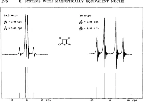
FIG. 6.4. E x p e r i m e n t a l a n d theoretical spectra for t h e p r o t o n s in p u r e 2 - b r o m o - 5 - c h l o r o t h i o p h e n e .

not conserve the total spin quantum number are strictly forbidden. T h e only transitions satisfying the selection rules ΑΙ = 0, Am = — 1 , are

ι ++>-^{i +-> + I -+»> ^{i +-> +1 —>•

T h e energy corresponding to the eigenvector with I = 1, m = 0, is the arithmetic mean of the energies corresponding to the eigenvectors with I = 1, m = ± 1, so that only a single resonance is observed, although two transitions are allowed.

T h e experimental spectra of the protons in 2-bromo-5-chlorothiophene, as observed at 24.3 and 60 Mcps, are shown in Fig. 6.4. T h e theoretical spectra for J/8 = 0.416 and 1.02 are added for comparison with the experimental traces. T h e ratio of the observed internal chemical shifts is 3.88/9.52 = 0.408, in good agreement with the ratio 24.3/60 - 0.405.

2. The A²B System A. Diagonalization of the Hamiltonian Matrix

T h e A²B system represents the next step in complexity beyond the simple AB system and provides an opportunity to apply the theory of magnetically equivalent nuclei to a nontrivial case.

2. T H E A2B S Y S T E M 197 T h e magnetic equivalence of the A nuclei demands the conservation of the total angular momentum of group A, which in turn implies the conservation of the total spin quantum numbers. Since group A contains two spin-^ nuclei, the values of IA are 1 and 0, each with spin multiplicity equal to unity. The product kets for group A will be denoted | 1, 1>, I 1, 0>, I 1, - 1 > , I 0, 0>, those for group Β, | 1 , £>, | \, - £>. T h e eight possible products of these kets, which provide a basis for the joint system, are given in Table 6.3.

T A B L E BASIS VECTORS FOR

6.3

THE A2B S Y S T E M

1 Ά = ^{0 m}

H,I; ¹ _2> ³ 2

1 1 , 1 ; ¹ _2> . - * > , ^{I 1,0;} i

t>

I

! 1, - 1; Ι ±\

2> 2 / > 1 1,0; J, -i> 1 0, 0; I -Έ> - I

I I, - I ; ¹ 2 '

-*

Operating on the elements of the product basis with Jif, one finds that the two product kets with IA = 1, m = ± F > and the two product kets with IA = 0, m = ± J > a r e eigenvectors of J^. T h e corresponding eigenvalues are given in Table 6.4.

T h e kets with IA = 1, m = ± ^ , generate a pair of 2 X 2 submatrices of J F , so that the hamiltonian matrix has the form indicated in Fig. 6.5(a).

Thus the diagonalization of the hamiltonian matrix requires only the diagonalization of the submatrices

_ 1 (±ω^Β Λ / 2 \ 2\JV2 ±œ^A±8~j)'

T h e results are given in Table 6.4, where the following notational abbreviations have been introduced:

^ 1 . 0 —

0 1 . 0 =

(S² - J8 -f 9 Ri.-i = ( δ² + / δ + 9 /²/ 4 )^{1 / 2}. Ql.-l JV2

T h e basis employed in the solution of the eigenvalue problem led to a particularly simple decomposition of the hamiltonian matrix, but it

198 6. SYSTEMS WITH MAGNETICALLY EQUIVALENT NUCLEI

Eigenvector Eigenvalue

U,l;iè>

îTi—il 1.0;i,i> -öi.. I

i -i»

(1

Q* )./, tgi.o I 1, 0; J, i> + I 1, 1; i -|>} -*(»

- f / + *i .o)

1

{11,-l;iè>-0,.-i|l,O;i,-J» è(«>A + i/+

ci + e

,.,)"

1

( 1 +, )]/10

-{Oi.-ill,-l;i,i>

1(» A

i/-

|0,0 ;J,i> -i«B

3

2 1 •V

2 •V

1

"2

•V

•V

i

= o. 1

2 i

= o.

1

"2

(o) (b)

F I G . 6.5. D i r e c t s u m decompositions of t h e A2B h a m i l t o n i a n m a t r i x relative t o bases that diagonalize: (a) IA 2, IB 2, a n d /2 ; (b) Iz alone.

would not have been incorrect to use some other basis; for example, the basis {| + + +>> | + H >, | >}. Although this basis may appear to be rather more obvious than the one actually used, it does not lead to optimum factorization of the secular determinant. In fact, the matrix for 3tf would have the form shown in Fig. 6.5b. T h e blocks with

2. T H E A2B S Y S T E M 199 m = ^ \ are three-dimensional, so that one is confronted with a pair of cubic equations. It turns out that these cubics are easily factored into linear and quadratic equations, but the essential point here—and in more complicated systems—is that optimum factorization of the hamiltonian matrix is automatically achieved if the elements of the initial basis are eigenvectors of I^{A 2}, I^{B 2}, and I^z .

B. Spectra of A²B Systems

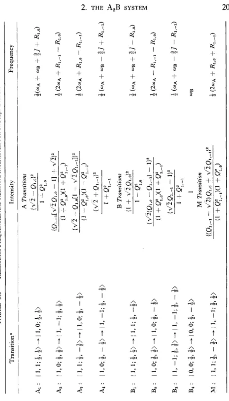
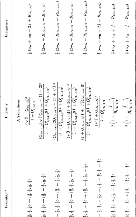
T h e spectrum of the A²B system is computed by the same procedure used for the AB system. In the present instance, transitions between states with different values of I^A are strictly forbidden. T h e resonance frequencies and their relative intensities are given in Table 6.5. T h e A transitions and the first three Β transitions conserve I^A = 1 ; B⁴ conserves

/ A = 0.

T h e last transition recorded in Table 6.5 is a mixed transition, that is, a transition with Am = AmA -f AmB = — 1, but with AmA and AmB

nonvanishing. Mixed transitions are not usually detected in the spectra of two-group systems since Int <^ Int A;, Int Bk (cf. the numerical data given in Appendix VI).

An interesting property of the A2B spectrum is that transition B4 leads to a resonance of unit intensity at the Larmor frequency of nucleus B.

Since the arithmetic mean of A2 and A3 is ωΑ , S = 1 { ( Α2 - B4) + (A, - B4)}.

T h e spin-spin coupling constant may be determined from the equation

/ = | { ( A , - A⁴) + (B, - B³)}.

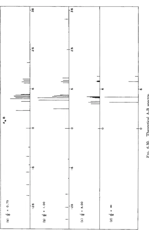
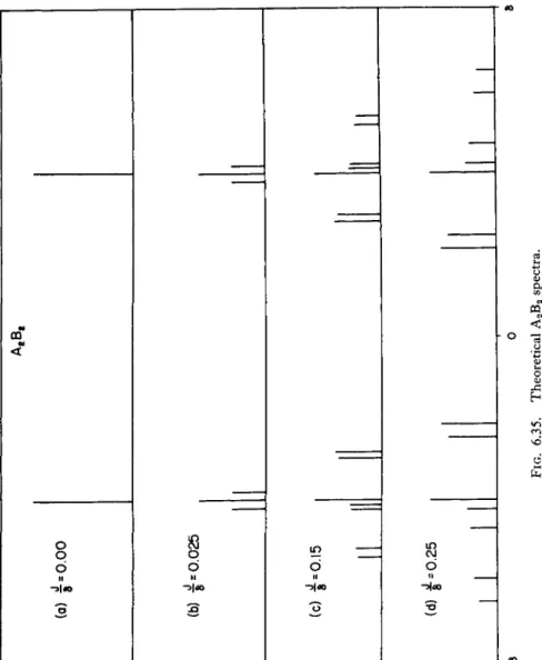
If all the A and Β transitions are not resolved / and δ are obtained by comparing the observed frequencies and integrated intensities with calculated spectra until the "best fit" is obtained. For this purpose, Figs. 6.6 through 6.8, and the numerical data in Appendix VI will be found most useful. Part (d) of Fig. 6.8 is drawn for δ Φ 0 and / infinitely large compared to δ. T h e three components of the symmetrical triplet are at zero (i.e., ωΒ), 2 δ/3, and 4 δ/3. When δ = 0, only a single resonance can be observed. An example of an A2B spectrum is shown in Fig. 6.9.

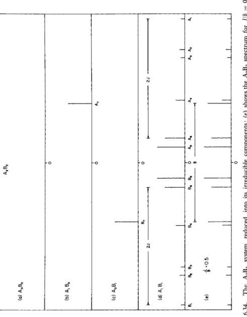
T h e A²B system is a reducible two-group system; its irreducible components are the A⁰B^{1 / 2} system, whose spectrum is the single resonance of unit intensity at ωΒ , and the A J B J / 2 system, whose spectrum makes up

200 6. SYSTEMS W I T H M A G N E T I C A L L Y E Q U I V A L E N T N U C L E I

A 2 B : ^ = 0 . 5

0

F I G . 6.6. T h e o r e t i c a l A2B s p e c t r u m for J/8 = 0.5. T h e frequency origin is at ωΒ .

( α ) j = ο

A 2 B

C ( b ) = 0 . 0 5

1

)

1

ί

c ( C ) ± = 0 . 1 5

1 ^{1 1}

1 6

i

( d ) -jf- = 0 . 2 5

ι I I 1

6

F I G . 6.7. T h e o r e t i c a l A2B spectra.

2. T H E A2B SYSTEM 201

J ^A 2 ^B

(0) ^{F =} 0.75

1 ι 1 ¹ -6 0 ι 1

(ω ^{I « ·}

1

I 1

8 28 -6 0 1

(O £ = 10

1 6 28

ι 1 1 -6 0 W)ï - ^s

1

6 26 1

— I

1

-6 0 6 28

the remaining eight lines of the A2B spectrum. T h e decomposition of the A2B system into its irreducible components is shown in Fig. 6.10 (the mixed transition is not shown).

T h e intensities of an A2B system satisfy the following relations:

Int Ai + Int

B

=

Int A⁴ + Int B³ = 3, Int A2 + Int A3 + Int B2 + Int M = 5.

T h e first two relations are deduced from the explicit expressions given in Table 6.5; the last relation follows from the first two and the fact that

IntAA/8

Additional examples of A2B spectra are provided by the 60 Mcps spectra of the — C H2O H protons of benzyl alcohol in acetone (Figs. 6.11 through 6.15). T h e chemical shift of the magnetically equivalent C H2

protons, relative to that of the hydroxyl proton, varies from 48.6 cps in pure benzyl alcohol to —7.8 cps for an acetone : benzyl alcohol volume ratio (VA/V^B) of 2.0. T h e coupling constant is 5.7 ± 0 . 1 cps and, within experimental error, independent of the acetone concentration. By varying the volume ratio, one can obtain spectra conforming to various

c p s *• 10

F I G. 6.9. E x p e r i m e n t a l a n d theoretical p r o t o n spectra of 1, 2, 3-trichlorobenzene in C S2 at 60 M c p s .

A0B±

1

-ε (

I

1

) I

ε

1

- 6 ( A2B = A , Bi + A0B i

I

1

) ε

-ε ο ε F I G . 6.10. R e d u c t i o n of t h e A2B system into its irreducible c o m p o n e n t s .

F I G . 6.11. E x p e r i m e n t a l a n d theoretical p r o t o n spectra of t h e m e t h y l e n e a n d h y d r o x y l g r o u p p r o t o n s of b e n z y l alcohol in acetone at 60 M c p s .

F I G. 6.12. E x p e r i m e n t a l a n d theoretical p r o t o n spectra of t h e m e t h y l e n e a n d h y d r o x y l g r o u p p r o t o n s of b e n z y l alcohol in acetone at 60 M c p s .

φCH

OH

• , ' 1 • • 1 1 • 1 '

-10 0 10 20 cps

F I G . 6 . 1 3 . E x p e r i m e n t a l a n d theoretical p r o t o n spectra of t h e m e t h y l e n e a n d hydroxyl g r o u p p r o t o n s of benzyl alcohol in acetone at 6 0 M c p s .

φCH

OH

£ * 1.4 Η 8=0

J

F I G . 6 . 1 4 . E x p e r i m e n t a l a n d theoretical p r o t o n spectra of t h e m e t h y l e n e a n d hydroxyl g r o u p p r o t o n s of benzyl alcohol in acetone at 6 0 M c p s .

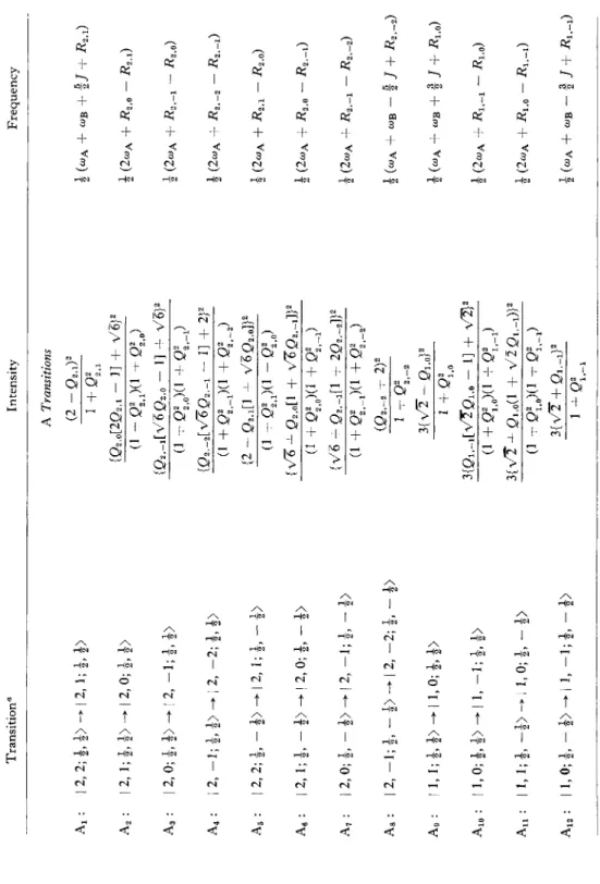
TABLE 6.5 — RESONANCE FREQUENCIES AND RELATIVE INTENSITIES FOR THE A2B SYSTEM Transition0 Intensity Frequency

A

: |l,l;ii>-|l ,0 ;|,i > A

: |l ,0 ;!,i>-|l , -1 ;ϋ > A

: |l,l;i-i>-|l ,0 ;i-i >

I

- i > - |

B,: |l,l;i,i>-|l,l;l,-1 > B

: I

I

B

: I 1 , -1 ; |,|>- > I 1 , - |> B

:

|, |> - I

A Transitions {V2 -g,,0}2 1 + ©;.· {Qi-i[V2Qi.. - H + V2}'

(1 + QJ

)(l + ρ* ^

Oi ,,)(l

{V2 + ft.-,}

{1 + V2Q

}

i(«A + ωΒ + fi + Äi.o) 1 (2ωΑ + Ält_! - jR1>0) \ (2ωΑ + Ä1>0 - R^) Η i (ωΑ + ωΒ - Î/ + Äi.-i) M

> ω

1

(2 <υ

φCH2OH

Η -

F I G. 6.15. E x p e r i m e n t a l a n d theoretical p r o t o n spectra of t h e m e t h y l e n e a n d hydroxyl g r o u p p r o t o n s of benzyl alcohol in acetone at 60 M c p s .

m

F I G. 6.16. S c h e m a t i c state d i a g r a m for t h e A2B system.

2. T H E A2B S Y S T E M 207 values of / / δ . In particular, one can observe the collapse of the spectrum to a single resonance when δ ^ 0 (Fig. 6.14), and the reversal of the ordering of the groups when δ changes sign (Fig. 6.15).

m

IA = I, W

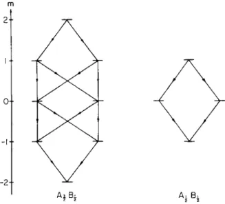
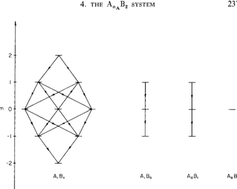
F I G . 6.17. T r a n s i t i o n d i a g r a m s for t h e i r r e d u c i b l e c o m p o n e n t s of t h e A2B system.

m

Α0Β± A, B|

F I G . 6.18. C o n v e n t i o n a l transition d i a g r a m s for t h e i r r e d u c i b l e c o m p o n e n t s of t h e A2B system.

208 6. SYSTEMS WITH MAGNETICALLY EQUIVALENT NUCLEI C. Transition Diagrams

A stationary state of an A²B system is defined by four eigenvalues:

Ω, m, I^A , and I^B . An arbitrary state of the system can be represented by a point ρ — (m, I^A , I^B , Ω) in a real four-dimensional space. Since nucleus Β is a spin-J particle, all states of the system have I^B = \ ; hence the points of the four-dimensional space can be projected onto points in a real three-dimensional space with coordinates (m, I^A , Ω).

T h e three-dimensional space is simply a "plane" of the four-dimensional space defined by the equation I^B = \. This projection yields the diagram shown in Fig. 6.16. This figure is purely schematic; no attempt has been made to indicate the correct relative magnitudes of the energies. T h e states of the system with I^A = 0 or I^A = 1 lie in the (two-dimensional) planes defined by these equations. T h e tie lines represent transitions satisfying the selection rules ΔΙ^Α = 0, Am = — 1.

T h e selection rule ΔΙ^Α = 0 prohibits the existence of tie lines connecting points in the plane I^A = 0 to points in the plane I^A = 1.

T h e state diagram may be simplified by drawing separate graphs for the planes I^A = 0 and I^A = 1, as shown in Fig. 6.17. A further simpli- fication results if one abandons the attempt to indicate differences in energies and adopts the symmetrical arrangements shown in Fig. 6.18.

In this figure the points representing the states of the system have been expanded to finite line segments to suggest energy levels. However the description of such figures as "energy-level diagrams" is not correct;

henceforth figures of this type will be called "transition diagrams."

A. The Structure of the Hamiltonian Matrix

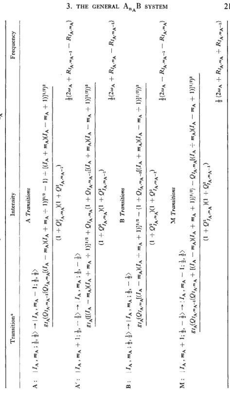
T h e AB and A²B systems are special cases of the AUAB system. T h e latter system provides an excellent illustration of the power and elegance of the concept of a group of magnetically equivalent nuclei. With the aid of this concept, exact recursive formulas for the resonance frequencies and line intensities can be derived for any value of nA whatsoever.

T h e conservation of the total angular momentum for group A permits the description of its spin states in terms of the total spin quantum numbers

3. The General Aⁿ Β System

k = 0, 1, 2, -|wA FOR nA EVEN,

0, 1, 2, I£-(wA — 1) FOR nA ODD, ^(3.1)

3. T H E G E N E R A L A„ Β S Y S T E M

209

with spin multiplicities

" JFLA-k+Wkl n^Al ^{( » a}

-26 + 1)

* 7 A F„ . A I 1 Μ Α Ι \ 3 ·Δ)

A generic ket for group A will be denoted | IA , mA}. T h e spin multi- plicity indices, î^{/ a} = 1, 2, -~>gi^A > need not be indicated in the kets for group A since the manner in which they enter the problem will be explicitly taken into account in the following discussion. However, one must keep in mind that there are 21^A + 1 kets for each choice of S^{I A} .

T h e conservation of I^{B 2} is ensured by using {| - | , -|>, | —1->}

as a basis for the spin space of nucleus Β alone. A basis for the spin space of the joint system is provided by the 2^{n A +1} independent product kets

{|/a,*a>Ü,±£>}

(3.3)

whose elements are simultaneous eigenvectors of I^{A 2}, I^{B 2}, and I^z. T h e hamiltonian matrix is not diagonal with respect to the basis

(3.3),

but it is easy to describe its structure. Since I^{A 2} is a constant of the motion, the matrix elements of connecting states with different values of I^A vanish, as indicated in Fig. 6.19 for n^A = 3. T h e only nonvanishing matrix elements of Jif are enclosed by the square blocks along the principal diagonal. Each of these "I^A blocks" is generated by product kets with the same value of I^A . T h e number of I^A blocks is equal to the number of distinct values of I^A ; hence

u er κι ι (J«A + 1 for «^Ae v e n ,

number of I^A blocks = f, ,_{^(n ^{1N r} , , (3.4)

A + l) for nA odd.

T h e product kets which generate an I^A block may be partitioned into g^lA sets of 2(2/^A + l ) members; each set is characterized by a distinct value of the spin multiplicity index s£ , as shown in Fig. 6.20. T h e nonvanishing matrix elements within an IA block are enclosed by the g^lA subblocks along the principal diagonal. Each of these subblocks is generated by a subset of the basis, formed by taking the (Kronecker) product of the 2/^A + l group-A kets with a fixed value of SJ and the two product kets for group B. T h u s the dimension of each subblock is 2(2/^A + l ) . Since there are gÎA subblocks, it follows that the dimension of an I^A block is 2gj^A(2I^A + l ) .

T h e submatrices enclosed by the gj subblocks of an I^A block are generated by sets of product kets described by the same quan- tum numbers. By suitably ordering the elements in the gj sets {I > ; O l h ± i>}> il 7A .^M A ; 2>| \ ; ± £>} ···, all these submatrices

210 6. S Y S T E M S W I T H M A G N E T I C A L L Y E Q U I V A L E N T N U C L E I

-2

F I G . 6. 1 9 . S t r u c t u r e of t h e hamiltonian F I G . 6. 2 0 . E a c h IA block of t h e h a m i l t o - m a t r i x for t h e A3B system. nian m a t r i x for t h e A „AB system factors into

S iA identical subblocks.

will be identical, so that one need only consider the structure of the submatrix enclosed by an arbitrary subblock. T o this representative sub- block one may apply the condition that the matrix elements of connecting states with different values of m = m^A + m^B must vanish.

T h e number of product kets corresponding to a given value of m in a typical subblock (— IA — ^ < m < IA -f may be determined by first choosing any product ket, say

11

,

If there is another product ket in the set of 2(21A + 1 ) kets {I I^A , m^A ; \R, ± J ) } with the same value of my the value of mB must be

— \ , since otherwise the second product ket would be identical with the product ket already selected. It follows that there are at most two product kets corresponding to the Iz eigenvalue m = mA + \ :

11

;

— i >

The second ket is not defined when m^A — I^A . This means that there is only one product ket with m = IA + \ , and it is an eigenvector of £F.

Similarly, when mA = —IA — 1, the first ket is undefined, and the second ket is an eigenvector of corresponding to m = —I^A — \ .

The substructure of a typical subblock of an I^A block is now easily described. It commences with a 1 X 1 matrix in the upper left-hand

3. T H E G E N E R A L A„ Β S Y S T E M

NA 211

corner, followed by a string of 2I^A 2 x 2 matrices along the principal diagonal, and terminates with a final l x l matrix in the lower right- hand corner (Fig. 6.21). T h e diagonalization of this subblock will be reduced to the solution of a single quadratic equation.

F I G . 6 . 2 1 . S u b s t r u c t u r e of t h e gj subblocks.

B. Diagonalization of the Hamiltonian Matrix

T h e 2 x 2 submatrix generated by the product kets (3.5) is obtained by operating on these kets with Jf⁷. One finds that

JP(IA , « A + I)

= _ 1 / (2ωΑ + J)mA + CUB J[(IA — » A ) ( / A + A M

2 \J[(IA - m^A)(I^A + m^A + 1)]^ (2a>^A ~ ]){m^A + 1) T h e eigenvalues and eigenvectors of this matrix are

Ω^Χ(Ι^Α , m^A + J ) = — | [ ( 2 m^A + 1) ω^Α — \ ] — # /^Α. ™^Α] , Ω²(Ι^Α, « A + i ) = - £[(2mA + 1) ωΑ - £ / + * /^Α. ™^Α] , I/ A , # * Α +

i ;

= " ( Γ + ρ | —J Ï 7 2 "( I ^{/ a} » ^{W A} ; i ' i > - Ö/A, mA I / A , WIA + l ; i ,

I

i ;

= ^ ρ ! Γ]2 I Ö / A . W A I / A , W A ; i , i > + I / A , W A + 1 ; -g-, +

+ 1 ) ]^{1 / 2}\ (3.6)

(3.7)

(3.8)