Sándor Bozóki
Computer and Automation Research Institute, Hungarian Academy of Sciences (MTA SZTAKI);
Department of Operations Research and Actuarial Sciences Corvinus University of Budapest
Budapest, Hungary
E-mail: bozoki@sztaki.hu, sandor.bozoki@uni-corvinus.hu Linda Dezső
University of Szeged;
International Study Programs, Corvinus University of Budapest Budapest, Hungary
E-mail: linda.dezso@gmail.com
József Temesi
Department of Operations Research and Actuarial Sciences Corvinus University of Budapest
Budapest, Hungary
E-mail: jozsef.temesi@uni-corvinus.hu
Attila Poesz
Department of Operations Research and Actuarial Sciences Corvinus University of Budapest
Budapest, Hungary
E-mail: attila.poesz@uni-corvinus.hu
ABSTRACT
Our research focused on testing various characteristics of pairwise comparison (PC) matrices in controlled experiments. About 270 students have been involved in the test exercises and the final pool contained 450 matrices. Our team conducted experiments with matrices of different size obtained from different types of MADM problems. The matrix elements have been generated by different questioning orders, too. The cases have been divided into 18 subgroups according to the key factors to be analyzed.
The testing environment made it possible to analyze the dynamics of inconsistency as the number of elements increased in a given case. Various types of inconsistency indices have been applied. The consequent behavior of the decision maker has also been analyzed in case of incomplete matrices using indicators to measure the deviation from the final ranking of alternatives and from the final score vector.
Keywords: multi-attribute decision making, pairwise comparison matrix, inconsistency, ranking
Corresponding author
1. Introduction
Pairwise comparison matrices are widely used in solving multi-attribute decision making problems.
However, in the past there has been a debate about the inconsistency derived from pairwise comparisons.
Most papers followed Saaty’s approach [Saaty, 1980] using his inconsistency index based on randomly generated matrices. One of the first studies on empirical PC matrices [Gass and Standard, 2002] pointed out important differences between randomly generated and experimental matrices. One of the aims of our empirical research was to generate a large number of PC matrices in a controlled test environment , and to analyze their inconsistency. Other debated questions in the MADM literature are the estimation and the stability of the weight/score vector, and the problem of rank reversal. Our research contributes to the discussions with some empirical evidences. This paper demonstrates the first results of the research.
2. Methodology
2.1 Some properties of PC matrices
In a MADM problem A = [aij]i,j=1…n pairwise comparison matrix is called consistent if and only if transitivity aij*ajk = aik holds for all i, j, k = 1,…n , otherwise it is called inconsistent. There are several inconsistency indices, but Saaty’s inconsistency index CR is the most frequently used one. CR is a positive linear transformation of the Perron eigenvalue λma x as follows: CR = (λmax – n)/(RIn*(n – 1)), where RIn is defined as (Λmax – n)/(n – 1), where Λmax is an average value of the Perron eigenvalues of randomly generated n×n PC matrices.
Another inconsistency index is based on 3×3 PC matrices [Koczkodaj, 1993]. The PC matrix of size 3×3, called triad, can be written in the following way:
1 c / 1 b / 1
c 1 a / 1
b a 1
CM inconsistency of a triad is defined as
a
c b c ,1 ac b b ,1 c a b a min 1 ) c , b , a ( CM
.
Furthermore, the extension of CM for higher dimension [Bozóki, Rapcsák, 2008] can be written by using the maximum function over the set of the triads as
CM(a ,a ,a ) 1 i j k n
.max ) A (
CM ij ik jk
In our further analysis we will use the generalization of PC matrix to the incomplete case. According to Harker [1987], an incomplete PC matrix contains one or more missing elements. Note that every (complete) PC matrix is built up through the series of incomplete PC matrices as follows: whenever the decision maker gives a matrix element, the number of missing elements decreases by one until the PC matrix has no missing values, i.e. becomes complete. Both the Eigenvector Method and the inconsistency index CR have been extended to incomplete PC matrices [Bozóki, Fülöp, Rónyai, 2010]. Inconsistency index CM has been as well generalized for the incomplete case [Bozóki, Fülöp, Koczkodaj, 2011]. Our calculations for incomplete matrices apply the algorithms introduced in these cited papers.
AHP and similar methods often use PC matrices for determining the scores of alternatives with respect to a given criterion, or determining values of a weight vector. One important question how these vectors will change if one or more alternatives/criteria are added or deleted. It is a widely held view that the (1)
(2)
(3)
occurrence of rank reversal in a weight vector is a drawback for a certain method. In this research we will not analyze rank reversal in a general context. Regarding scores of alternatives and ranks of alternatives our research concentrates on the incomplete case. The decision maker builds up the PC matrix step by step (answering questions one by one). In our experiments we recorded each answer for each question for each subject in the process, thus we could calculate scores in each step. If the scores calculated from the final (complete) matrix are different from the scores determined after a sequence of steps we can use indicators to evaluate the consequent behavior of the decision maker.
One indicator can be obtained by comparing the ranks of the alternatives determined from the complete PC matrix to the rankings derived from the incomplete matrices. For this purpose we calculated the number of rank reversals and the Spearman rank correlation coefficient. Another indicator is the Euclidean norm computed for the score vector obtained from an incomplete matrix after a certain number of questions in the procedure, and the final one.
2.1 Research questions and the experime ntal design
Our research combined the experimental techniques with mathematical and statistical tools to analyze some research questions. A few of them are listed here:
Q1. Are the inconsistency indices systematically higher in case of subjective type of problems?
Q2. Are the inconsistency indices higher in case of large size PC matrices?
Q3. Has the questioning method an impact on the inconsistency?
Q4. Is the behavior of the decision maker consequent in the course of the whole questioning procedure?
Q5. What can we say about inconsistency and the weight vector if both are computed from incomplete data?
After a thorough preparation controlled tests have been run with the help of student groups volunteering at participating in the experiment. About 270 business and economics students have been involved in the test exercises. We had groups of 22-26 students in each experiment.
The low level of inconsistency of a pairwise comparison matrix is very important to guarantee the right results to obtain scores, weights, or preferences from the PC matrix. One of the research questions was the sensitivity (volatility) of inconsistency indices CR and CM for changes of different characteristics. For this purpose the dimensions of the test problems were: size, type of the problem, order of questioning, and completeness. The size of the matrices were 4×4, 6×6 and 8×8. The experimental design made possible to trace and to analyze the properties of incomplete matrices in the order of the questions, too. The answer sheets wee presented in small leaflet with one question on every page. In this way subject answered the questions in a predetermined order.
For obtaining the elements of the matrix standard elicitation techniques have been developed. These techniques ensure some significant properties of the PC matrices (e.g. reciprocal property), and their scales are calibrated to meet the requirements of the given decision-making method (1 to 9 scale in case of the AHP, for instance). Verbal and numerical scales have been applied. When the elements of the PC matrix are determined one by one, we will refer to it as a “questioning procedure”. Questioning can be executed either by the assistance of decision-aiding experts, or by a decision support system without the presence of a decision-aiding person. In our experiments the subjects filled in the PC matrices for a given problem following our instructions, but without any interaction. According to the size of the PC matrix the decision makers (subjects of the experiments) had to answer at least 6 (size 4×4) and at most 28 (8×8) questions. The questioning order of a particular procedure will be described later.
In our empirical research we designed different test environments in order to analyze the research questions. One group of the tests has been designed to investigate the impact of the nature (type) of the
problem. The quality of the applied stimuli (the test problems) was categorized into “subjective” and
“objective” groups based on our previous validation: the participants answered pairwise comparison questions in problems of comparing the size of countries on a map (“objective” type), and comparing summer houses (“subjective” type). Note, that we used an imaginary map with irregular contours of the countries.
For the “objective” stimuli, subjects were asked to compare every pair of the presented countries by their size. First, subjects had to indicate which country is larger. Then, they had to indicate by how much it is larger. Thus, if one country was judged 30% larger than the other it was indicated to be 1.3 times larger.
For the “subjective” stimuli subjects were asked to state which summer house they like more, and how much more they like it. For the latter they were given the verbal scale proposed by Saaty [Saaty, 1980].
Every subject was presented with one subjective and one objective set of stimuli (i.e. every group filled in two PC matrices of different types), and the order of the presentation (that is whether “subjective” stimuli was given first or second) was randomly assigned to each subject. The stimuli were administered within three conditions. The first condition was the order of the presented stimuli as detailed above. The second condition was the size of the matrices: 4x4, 6x6 and 8x8. In one session we have applied one size for the whole sample.
The third condition implied the questioning procedure. In the first group of cases the countries were compared in random order. In the second group a sequential order was used: country number one was first compared to country number two, then to number three, etc. In the third group Ross-type comparison [Ross, 1934] was applied. Ross constructed an order optima lly balanced for two conditions: i) maximizing the time of reappearance of the same item, ii) the number of 1st positions and the 2nd positions in the comparisons should be as close to each other as possible for every item.
That way the whole sample has been divided into 18 subgroups as it is seen in the example of Table 1 for a 6×6 matrix. A, B, C, D, E, F denote the alternatives.
Table 1. Fill-in order of a 6x6 matrix
question order
1. 2. 3. 4. 5. 6. 7. 8. 9. 10. 11. 12. 13. 14. 15.
sequential A-B A-C A-D A-E A-F B-C B-D B-E B-F C-D C-E C-F D-E D-F E-F Random A-F B-E A-C F-E C-D B-D B-F A-E C-E A-D E-D C-F B-C A-D B-A Ross A-B F-D E-A C-B E-F A-C B-D F-A D-C E-B A-D C-E B-F D-E C-F
3. Results
Several calculations have been made using MATLAB and SPSS. In this paper we are focusing on two major issues. First we explore whether the changes of the inconsistency indices show any patterns throughout the different test environments? Second, we will be analyzing the incomplete matrices.
3.1 Inconsistency indices
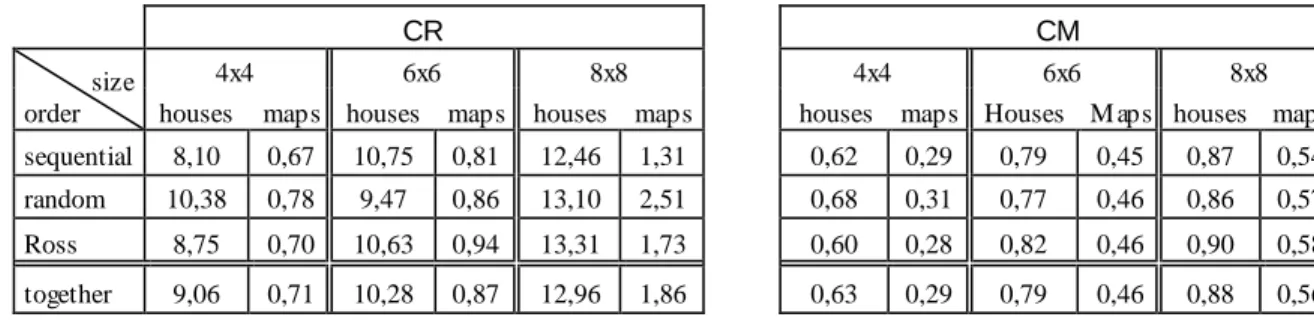
For all complete PC matrices the CR inconsistency index has been calculated. As we described above the matrices differed in size, in questioning order and in the type of the problem. A great number of result tables could have been constructed. In Table 2, for instance, where the discriminating factor was the type of the problem, we could draw conclusions about the impact of the size and the questioning order. The first part of the table contains the CR averages of 450 matrices. One cell is the average of 22-26 matrices.
Table 2. The average of CR and CM inconsistenc ies (in %) in case of complete matrices
CR CM
size order
4x4 6x6 8x8 4x4 6x6 8x8
houses maps houses maps houses maps houses maps Houses M aps houses maps sequential 8,10 0,67 10,75 0,81 12,46 1,31 0,62 0,29 0,79 0,45 0,87 0,54 random 10,38 0,78 9,47 0,86 13,10 2,51 0,68 0,31 0,77 0,46 0,86 0,57 Ross 8,75 0,70 10,63 0,94 13,31 1,73 0,60 0,28 0,82 0,46 0,90 0,58 together 9,06 0,71 10,28 0,87 12,96 1,86 0,63 0,29 0,79 0,46 0,88 0,56
Recall that in Q1 we predicted that the inconsistency index will be higher for subjective problems. As it can be seen from Table 2 the inconsistency index averages are around 10% (or above) in case of scoring summer houses (first columns for each size), and the same averages are about 1% for the map problems (second columns for each size). According to our expectations the CR indices are significantly higher for a problem of subjective nature (how much one house is more appealing than the other) than for a problem of objective type (how much one country is larger than the other).
Furthermore CR index is (almost) monotonically increasing for both types of stimuli: the larger is the size the larger of the CR index is irrespective of the questioning order. The empirical evidence shows a very stable tendency (there is only one exception in our table) as we predicted in Q2.
We can mention that the decision makers were very close to Saaty’s 10% acceptance rule (at least looking at the averages) in the case of the subjective type of the problem (for each size and for each questioning order); the 8×8 matrices even produced higher values than 10%.
We also calculated the CM index for the same matrices. The results can be seen in the second part of Table 2. In case of interpreting CM index we have information about the order and the magnitude of the differences (like in case of the CR). The data in the second part of Table 2 (CM) confirm the tendencies obtained from the first part of Table 2 (CR).
Note that CM threshold for acceptance has been defined for a very special case (CM ≤ 1/3 is proposed for 4×4 matrices with elements from the ratio scale 1-5 [Koczkodaj, Herman, Orlowski, 1997]), therefore a more exact interpretation of CM values is subject of future research.
A novelty of our research was to analyze the impact of the questioning order. Without any previous experience our hypothesis was (see Q2) that one of the questioning methods (e.g. the sequential method) can produce significantly better (lower) CR values than the others. The data in our Table 2 do not support that hypothesis: we could not detect systematic differences derived from the questioning order.
3.2 Analysis of the inc omplete matrices
One way to test the consequent behavior of a decision maker (Q4) is a step by step tracking of respondents’ answers in the questioning procedure. This allows us not only to measure/index the inconsistency at the end of the procedure but to locate where the inconsistency emerged (see more details in [Bozóki, 2011]. As an example of such kind of analysis we show first Tables 3a and 3b. The “number of matrix elements” implies the number of answered questions. In case of 6×6 matrices the range is from 5 to n(n – 1)/2 = 15. CR inconsistencies can be calculated in each case [Bozóki, Fülöp, Rónyai, 2010] and their averages are included in the respective cell. The tables contain results for each questioning order separately.
Table 3. The average of CR inconsistencies (in %) in case of 6×6 incomplete matrices
Table 3a. Summer houses
number of matrix elements Order
5 6 7 8 9 10 11 12 13 14 15
Sequential 0,00 0,96 1,82 3,71 4,74 5,66 6,61 7,33 8,35 9,21 10,75
Random 0,01 1,38 2,77 3,49 4,42 4,97 6,25 6,91 8,17 8,19 9,47
Ross 0,01 1,37 2,50 3,84 4,93 5,45 6,27 7,24 7,85 9,52 10,63
Table 3b. Maps
number of matrix elements Order
5 6 7 8 9 10 11 12 13 14 15
Sequential 0,00 0,13 0,18 0,25 0,32 0,40 0,48 0,55 0,64 0,72 0,81
Random 0,01 0,06 0,11 0,21 0,40 0,51 0,58 0,66 0,72 0,73 0,86
Ross 0,00 0,07 0,14 0,23 0,31 0,37 0,50 0,73 0,79 0,89 0,94
The elements of the last columns are equal to the respective elements from the first part of Table 2. From the analysis of Table 2 we know that there are significant differences in the CR averages comparing the values of the summer house and the map problems. Table 3 gives evidences that from 0 to the final CR value the averages demonstrate a monotonic increase. As the CM inconsistency analysis brought similar results, we do not refer to them in details.
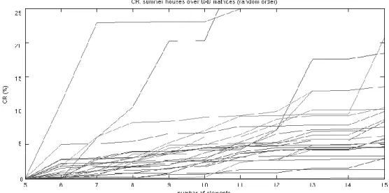
Figure 1 shows the consequent behavior of the decision makers individually by their CR values. All broken lines in the figure denotes one subject in the group. If we draw a vertical line at every step (from 5 to 15) we will see the individual values of the CR inconsistency after having answered that number of questions. This figure gives details about the averages in the second row of Table 3a.
Figure 1. The individual CR inconsistencies in case of 6×6 matrices, random questioning order
Figure 1 demonstrates that the behavior of the subjects – monotonic increase in CR – is the same as we concluded for the averages. One can also note that in this group (25 subjects) only 8 of them had CR index higher than 10%.
Another way to check the consequent behavior of the decision makers is to trace the number of rank reversals in each step (i.e. in the subsequent incomplete matrices). We calculated the score vectors in each step and they generated a ranking of the alternatives in each step. Then we compared the final ranking to those ones obtained in the course of the questioning procedure. Our summer house and map tables show again the strong impact of the type of the problem: in case of the objective problem (25 subjects) only a very few of them had a different ranking compared to the final one.
We can compare the final ranking and the step by step rankings with the help of the Spearman rank correlation coefficient, too. The coefficient gives +1 if the ranks are identical, and gives – 1 if they are totally in contradiction. Table 4 contains Spearman coefficients for the 6×6 matrices.
Table 4. Spearman rank correlation coefficients in case of 6×6 incomplete matrices
number of matrix elements Type
5 6 7 8 9 10 11 12 13 14 15
summer houses 0,82 0,88 0,90 0,92 0,93 0,94 0,96 0,97 0,97 0,98 1,00 M aps 0,97 0,97 0,98 0,98 0,98 0,98 0,99 0,99 0,99 1,00 1,00
The averages (and our detailed calculations) show that the initial rankings were not very far from the final ranking for the majority of the decision makers – of course, again, there was a difference caused by the type of the problem.
4 Conclusions
Our team generated empirical pairwise comparison matrices to analyze some research questions. Our view was that the great number of matrices obtained from controlled experiments could be a solid basis to draw conclusions about the properties of PC matrices. The first results are demonstrated in this paper.
One group of the results justified that the type of the problem and the size of the problem have impacts on the inconsistency indices. We also investigated the impact of the questioning order and significant impact has not been found. As the analysis of the questioning order (and some other features of the questioning methods) have not been in the forefront of previous research, more facts are needed to describe their potential influence. Our future plans include experiments to explore the impact of the range of the scale, and the impact of the applied techniques (verbal, visual, quantitative) based on the data from empirical matrices, as well.
In real-world applications incomplete PC matrices can occur. Some research papers have already published results about this topic, however, a lot of unexplored territories remained. This paper gives our preliminary results based on incomplete matrices generated by a step by step procedure. New techniques have been applied to answer our questions about the behavior of the decision maker in the course of eliciting the elements of the PC matrix. Our future tests intend to contribute to the discussion about the right number of matrix elements for MADM methods based on pairwise comparison matrices, too.
REFERENCES
Bozóki, S. (2011). An inconsistency control system based on incomplete pairwise comparison matrices, Proceedings of The International Symposium on the Analytic Hierarchy Process (ISAHP), 15-18 June, 2011, Sorrento (Naples), Italy.
Bozóki, S., Fülöp, J., & Rónyai, L. (2010). On optimal completions of incomplete pairwise comparison matrices, Mathematical and Computer Modelling, 52, 318-333.
Bozóki, S., & Rapcsák, T. (2008). On Saaty’s and Koczkodaj’s inconsistencies of pairwise comparison matrices, Journal of Global Optimization, 42(2), 157-175.
Gass, S.I., & Standard, S.M. (2002). Characteristics of positive reciprocal matrices in the analytic hierarchy process, Journal of the Operational Research Society, 53(12), 1385-1389.
Harker, P.T. (1987). Incomplete pairwise comparisons in the analytic hierarchy process, Mathematical Modelling, 9(11), 837-848.
Koczkodaj, W.W. (1993). A new definition of inconsistency of pairwise comparisons, Mathematical and Computer Modelling 8, 79-84.
Koczkodaj, W.W., Herman, M.W., & Orlowski, M. (1997). Using consistency-driven pairwise comparisons in knowledge-based systems. In: Proceedings of the Sixth International Conference on Information and Knowledge Management, 91-96. ACM Press.
Ross, R.T. (1934). Optimum orders for the presentation of pairs in the method of paired comparison, Journal of Educational Psychology, 25, 375-382.
Saaty, T.L. (1980). The analytic hierarchy process, McGraw Hill, New York