Does timing of decisions in a mixed duopoly matter?

(will be inserted by the editor)

Does Timing of Decisions in a Mixed Duopoly Matter?

Tam´as L´aszl´o Balogh · Attila Tasn´adi

Received: date / Accepted: date

Forthcoming in theJournal of Economics (2012).

Springer-Verlagc ¹

Abstract We determine the endogenous order of moves in a mixed price- setting duopoly. In contrast to the existing literature on mixed oligopolies we establish the payoff equivalence of the games with an exogenously given order of moves if the most plausible equilibrium is realized in the market. Hence, in this case it does not matter whether one becomes a leader or a follower. We also establish that replacing a private firm by a public firm in the standard Bertrand-Edgeworth game with capacity constraints increases social welfare and that a pure-strategy equilibrium always exists.

Keywords Bertrand-Edgeworth, mixed duopoly, timing games JEL ClassificationsD43, L13

T.L. Balogh

University of Debrecen, Department of Economic Analysis and Business Informatics, H-4028 Debrecen, Kassai ´ut 26.

Tel.: +36-52-416580/77068 Fax: +36-52-419728

E-mail: tamas.balogh@econ.unideb.hu A. Tasn´adi

Department of Mathematics, Corvinus University of Budapest, H-1093 Budapest, F˝ov´am t´er 8, Hungary

Tel.: +36-1-4827442 Fax: +36-1-4827430

E-mail: attila.tasnadi@uni-corvinus.hu

1 The original article is available at www.springerlink.com. DOI: 10.1007/s00712-011- 0252-6

1 Introduction

The early literature on mixed oligopolies considered games with a predeter- mined order of moves and investigated market regulation possibilities through a public firm, especially, in order to increase social welfare. For instance, Cremer et al (1989) analyze the regulation of a simultaneous-move quantity- setting oligopoly market for which they report that the market outcome is equivalent to the solution, in which the central authority maximizes total surplus subject to the constraints that the public firms must break even.

Fraja and Delbono (1989) show for a mixed quantity-setting homogeneous good oligopoly that public leadership leads to higher social welfare than the simultaneous-move mixed or standard oligopolies.² However, comparing the simultaneous-move case with or without a public firm leads to an ambivalent result: It can happen that if there are sufficiently many identical firms on the market, then the public firm is better advised to maximize its profits in order to increase social welfare. Remaining in the quantity-setting framework, Cor- neo and Jeanne (1994) derive conditions under which the presence of a public firm can be beneficial.³

In a seminal paper Pal (1998) investigates for mixed oligopolies the en- dogenous emergence of certain orders of moves.⁴Assuming linear demand and constant marginal costs, he shows for a quantity-setting oligopoly with one public firm that the simultaneous-move case does not emerge, the public firm as a first mover emerges just in the two-period duopolistic case, while the pri- vate firms moving simultaneously in the first period followed by the public firm in the second period always constitutes a subgame-perfect Nash equilibrium of the timing game. His main observations are that incorporating a public firm substantially changes the outcome of the timing game and that the presence of a public firm increases social welfare.⁵ Matsumura (2003) relaxes the assump- tions of linear demand and identical marginal costs employed by Pal (1998).

The case of increasing marginal costs in Pal’s (1998) framework has recently been investigated by Tomaru and Kiyono (2010).⁶

There is less literature on price-setting mixed oligopolies. Ogawa and Kato (2006) consider mixed duopolies in the framework of a homogeneous good

2 We will frequently refer to oligopolies without public firms as standard or purely private oligopolies.

3 For other notable contributions in these directions, see for instance, Harris and Wiens (1980), Beato and Mas-Colell (1984) and Anderson et al (1997).

4 The timing question in purely private oligopolies has been investigated earlier by Gal- Or (1985), Dowrick (1986), Boyer and Moreaux (1987), Hamilton and Slutsky (1990) and Deneckere and Kovenock (1992), among others.

5 Jacques (2004) noted that in the duopolistic case with more than two periods the public firm producing in the first period and the private firm producing in the last period is also a subgame-perfect Nash equilibrium. In addition, Lu (2007) shows for the duopolistic case there are even more subgame-perfect Nash equilibria in which the private firm can produce in any period with the exception of the last one and the public firm has to produce in a subsequent period.

6 For further extensions we refer to Anam et al (2007) and Lu and Poddar (2009), among others.

price-setting game. They investigate a symmetric Bertrand duopolistic set- ting in which the firms have to serve the entire demands they face. Assuming linear demand and identical quadratic cost functions, they find for the two sequential-move games that the presence of a public firm may be either harm- ful or beneficial, while for the simultaneous-move game the outcome remains the same as shown by Dastidar (1995) for the purely private case. Dastidar and Sinha (2011) extend these results to strictly convex cost functions and decreasing demand functions. In another recent work Roy Chowdhury (2009) considers a price-setting mixed Bertrand duopoly (that is, firms have to serve the demands they face) and a mixed semi-Bertrand duopoly (in which only the public firm has to meet all demand). However, he focuses on the simultaneous- move case, and thus, does not solve the timing problem. For a heterogeneous goods price-setting mixed duopoly timing game B´arcena-Ruiz (2007) obtained the endogenous emergence of simultaneous moves.

In this paper we investigate a homogeneous good mixed Bertrand-Edgeworth duopoly with capacity constraints. In contrast to the literature on endogenous timing in purely private firm oligopolies as well as mixed oligopolies we find that the order of moves does not matter (Corollary 1). In addition, social wel- fare is higher in the mixed version of the Bertrand-Edgeworth game than in its standard version with only private firms (Corollary 2). As a byproduct we obtain that the mixed version of the Bertrand-Edgeworth duopoly game has an equilibrium in pure strategies for any capacity levels (Corollary 3).

The remainder of the paper is organized as follows. In Section 2 we present our framework and introduce the necessary notations. In Section 3 we recall the results of Deneckere and Kovenock (1992) on the capacity-constrained Bertrand-Edgeworth duopoly game with purely private firms, which we will need in comparing the results of the mixed version of the Bertrand-Edgeworth game with its standard version. Section 4 determines the equilibria of three games with exogenously given orderings of moves. Section 5 gathers the main consequences of our analysis carried out in Section 4. Section 6 illustrates our results in case of linear demand. Finally, we conclude in Section 7.

2 The framework

The demand is given by functionDon which we impose the following restric- tions:

Assumption 1 The demand function D intersects the horizontal axis at quantity a and the vertical axis at price b. D is strictly decreasing, concave and twice continuously differentiable on (0, a); moreover,Dis right-continuous at 0, left-continuous atband D(p) = 0 for allp≥b.

Clearly, any price-setting firm will not set its price aboveb. Let us denote byP the inverse demand function. Thus,P(q) =D⁻¹(q) for 0< q≤a,P(0) =b, andP(q) = 0 forq > a.

On the producers’ side we have a public firm and a private firm, that is, we consider a so-called mixed duopoly. We label the public firm with 1 and the private firm with 2. Our assumptions imposed on the firms’ cost functions are as follows:

Assumption 2 The two firms have zero unit costs up to their respective positive capacity constraintsk₁ andk₂.⁷

We shall denote by p^c the market clearing price and by p^M the price set by a monopolist without capacity constraints, i.e. p^c = P(k₁+k₂) and p^M = arg max_p∈[0,b]pD(p). In what follows p₁, p₂∈[0, b] stand for the prices set by the firms.

For all i ∈ {1,2} we shall denote by p^m_i the unique revenue maximizing price on the firms’ residual demand curvesD_i^r(p) = (D(p)−kj)⁺, wherej ∈ {1,2}andj6=i, i.e.p^m_i = arg max_p∈[0,b]pD_i^r(p). The inverse residual demand curves will be denoted by R1 and R2. Clearly, p^c and p^m_i are well defined whenever Assumptions 1 and 2 are satisfied.

Let us denote by p^d_i the price for which p^d_i min{ki, D p^d_i

}=p^m_i D^r_i(p^m_i ), whenever this equation has a solution.⁸Provided that the private firm has ‘suf- ficient’ capacity (i.e.p^c< p^m₂), then if it is a profit-maximizer, it is indifferent to whether serving residual demand at price levelp^m_i or selling min{ki, D p^d_i

} at the lower price levelp^d_i.

Concerning the employed rationing rule, we impose the following assump- tion.

Assumption 3 We assume efficient rationing on the market.

Thus, the firms’ demands equal

∆i(D, p1, q1, p2, q2) =







D(pi) ifpi< pj

Ti(p, q1, q2) ifp=pi=pj

(D(p_i)−q_j)⁺ifp_i> p_j

for all i ∈ {1,2}, whereTi stands for a tie-breaking rule.⁹ We will consider two sequential-move games (one with the public firm as the first mover and one with the private firm as the first-mover) and a simultaneous-move game.

An appropriate tie-breaking rule will be specified for each of the three cases.

We assume that the firms play the production-to-order type Bertrand- Edgeworth game, and therefore, the game reduces to a price-setting game since the firms can adjust their productions to the demands they face. Now

7 The real assumption here is that firms have identical unit costs since in case of production-to-order, as will be assumed later, this is just a matter of normalization.

8 The equation definingp^d_i has a solution if, for instance,p^m_i ≥p^c, which will be the case in our analysis when we will refer top^d_i.

9 The selection of the appropriate tie-breaking rule will ensure the existence of a Nash equilibrium or subgame-perfect Nash equilibrium in order to avoid the consideration of ε-equilibria implying a more difficult analysis without substantial gain.

we are ready to specify the firms objective functions. The public firm aims to maximize total surplus, that is,

π1(p1, p2) =

Z min{^(D(pj)−ki)⁺,k_j}

0

Rj(q)dq+

Z min{a,ki} 0

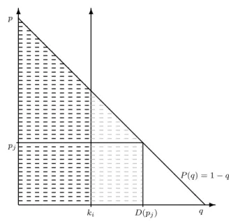
P(q)dq, (1) where 0 ≤ pi ≤ pj ≤ b. Figure 1 illustrates the social welfare, where the area indicated by black dashed lines corresponds to the second integral, while the area indicated by grey dashed lines corresponds to the first integral in expression (1). It should be mentioned that the first integral is not directly

Fig. 1 Social welfare

p

q- 6

@

@

@

@

@

@

@

@

@

@

@

@

@

@

@

@

@

@

P(q) = 1−q

6

ki

pj

D(pj)

drawn based onRj, but by a rightward shift of the vertical axis byki units, which enables us to illustrate the social welfare in one figure. It can be easily seen that in determining social welfare the low price does not play a role unless both prices are too high.

The private firm is a profit-maximizer, and therefore,

π2(p1, p2) =p2min{k2, ∆2(D, p1, k1, p2, k2)}. (2)

3 The benchmark

We will compare our price-setting mixed-oligopoly games with the price-setting games with purely private firms, that is, both firms’ profit functions take the form of the expression given by (2). The purely private case has been investi- gated by Deneckere and Kovenock (1992) from which we recall the interesting

case in which the simultaneous-move game does not have an equilibrium in pure strategies, i.e.,p^m₂ > p^cin case ofk2≥k1.¹⁰We shall emphasize that De- neckere and Kovenock (1992) assume for the sequential-move games that the demand is allocated first to the second mover¹¹and for the simultaneous-move case that the demand is allocated in proportion of the firms’ capacities.¹² Proposition 1 (Deneckere and Kovenock,1992)Underk2≥k1,p^m₂ > p^c and Assumptions 1-3, the results below are known about the equilibrium of the three games.

1. The simultaneous-move game only has an equilibrium in mixed strategies with common support [p^d₂, p^m₂] and equilibrium profits are equal to π₁^S = p^d₂k₁ andπ₂^S =p^m₂D^r₂(p^m₂) =p^d₂min{k₂, D p^d₂

}.¹³

2. If firm 2 moves first and firm1 second, then in a subgame-perfect equilib- rium the equilibrium prices are given by p₂ =p₁ =p^m₂ and the respective equilibrium profits equal π₂^L = p^m₂D₂^r(p^m₂) and π^F₁ = p^m₂ k1. In addition, if k1 = k2, then we also have a second subgame-perfect equilibrium with equilibrium prices given by p2=p^d₂ andp1=p^m₂.

3. If firm 1 moves first and firm 2 second, then in a subgame-perfect equi- librium the equilibrium prices are given by p1 =p^d₂ and p2 =p^m₂ and the respective equilibrium profits equalπ^L₁ =p^d₂k1 andπ^F₂ =p^m₂D^r₂(p^m₂). In ad- dition, if k1=k2, then we also have a second subgame-perfect equilibrium with equilibrium prices given by p1=p^m₂ andp2=p^m₂.

Deneckere and Kovenock (1992) find that firm 2 moving first and firm 1 moving second constitutes an equilibrium of the timing game, which can be verified by looking at the payoff table of a two-period timing game shown in Table 1, where in case ofk2> k1 we have π₁^F > π₁^S=π^L₁ andπ^L₂ =π^S₂ =π₂^F.

Table 1 Payoffs for the two period timing game.

First period Second period First period (π^S₁, π^S₂) (π^L₁, π₂^F) Second period (π^F₁, π^L₂) (π₁^S, π₂^S)

In addition, by introducing more time periods and discounting, Deneckere and Kovenock (1992) achieve that this ordering of moves is the one and only emerging endogenously.

10 For other cases the game reduces to the standard Cournot and Bertrand games.

11 This distinction ensures that the second mover does not need to slightly undercut the first mover.

12 It should be emphasized that the obtained results remain valid for a large class of other tie-breaking rules employed in the simultaneous-move game.

13 The results gathered in case 1 summarize the results obtained by Levitan and Shubik (1972), Kreps and Scheinkman (1983) and Osborne and Pitchik (1986).

4 Exogenously given order of moves

In our analysis we will discuss the above mentioned three games with exoge- nously given ordering of moves for the mixed duopoly version of the Bertrand- Edgeworth game. We are restricting ourselves again to the interesting case in which the simultaneous-move purely private version of the Bertrand-Edgeworth game does not have an equilibrium in pure strategies, i.e. max{p^m₁ , p^m₂}> p^c.¹⁴ Note that as there are two different types of firms (as far as their payoffs are concerned), it is not the same whether the private or the public firm has the higher capacity. In particular, we have to distinguish between the following two cases: (i) p^m₂ > p^c and (ii)p^m₁ > p^c ≥p^m₂. We will also refer to the first case as thestrong private firm case and to the second case as theweak private firm case. Therefore, we would have to analyze both cases separately for all the three orderings of moves.

4.1 The strong private firm case

Firstly, let us make clear that the pricep^d₂ having been defined earlier always exists sincep^m₂ > p^c. Therefore, we make no mistake if we use this price in our results in this section.

Now we collect some basic results in the following lemmas.

Lemma 1 Under Assumptions 1-3 and p^m₂ > p^c, it is in none of the timing games with an exogenously given order of moves optimal for the private firm to declare p2< p^d₂.

Proof We get the result directly from the definition ofp^d₂. By settingp2=p^m₂, even if the private firm serves only residual demand, its profit will be higher

than at a pricep2less than p^d₂. ut

Lemma 2 Under Assumptions 1-3 and p^m₂ > p^c, the social welfare in an equilibrium cannot be larger than the social welfare associated with the case in which both firms set pricep^d₂.

Proof The definition of the public firm’s profit implies that if a firm serves residual demand, then the lower price it sets the higher the social welfare.

On the other hand, if a company is the low-price firm, and it produces at its capacity limit, then changing its price, as long as it remains a capacity constrained low-price firm, does not alter social welfare. The private firm will not set its price belowp^d₂ by Lemma 1, while the public firm cannot increase social welfare by setting a price belowp^d₂. Hence, comparing all cases satisfying min{p1, p2} ≥ p^d₂, social welfare is maximized when both firms set price p^d₂. u t

14 Otherwise, the ordinary price-setting game results in a market-clearing or a competitive outcome, which also remains the outcome of the mixed duopoly game. For more details we refer to the concluding remarks in Section 7.

Lemmas 1 and 2 show that deleting strictly dominated strategies from the private firms strategy set excludes prices belowp^d₂ and after thatp^d₂ turns out to be a weakly dominant strategy of the public firm.

Now that we are aware of these results, we begin to discuss the three games with an exogenously given ordering of moves. We will start with specifying the tie-breaking rules for these games. The most common assumption if two firms set the same price, is that they share the consumers in proportion to their capacities (i.e. firmsi’s sales equal min{k_i, D(p)k_i/(k₁+k₂)}. Clearly, any of the two firms has the right to let its competitor serve a certain portion of its consumers. Such an act would seem to be irrational at first sight, but we will see below that if it is carried out by the public firm, it can drive the market to a socially better equilibrium. A more complete specification of the game would allow the public firm to select the consumers freely, strategically leaving them to the private firm. However, we fix a tie-breaking rule, which turns out to be compatible with the public firms incentives, and after determining the equilibria of the three games it can be easily verified that the public firm could not have selected a better tie-breaking rule.

Assumption 4 We specify the tie-breaking rules for the three games in the following way:

– In the simultaneous-move game we assume that if p1 = p2 ≤ p^d₂, then the demand is allocated first to the private firm (in other words: the public firm allows the private to serve the entire demand up to its previously given capacityk2). Otherwise the two firms share the consumers proportionally, i.e. firmi’s sales equal min{ki, D(p)ki/(k1+k2)}.

– Whenthe public firm is the first mover, we assume that the entire demand is allocated first to the private firm (i.e. to the second mover) at any price level in case of price ties.

– Provided that the private firm moves first, if p₁ = p₂ ≤ p^d₂, then the demand is allocated first to the private firm; otherwise the entire demand is allocated first to the public firm (i.e. to the second mover).

One can observe that for prices higher thanp^d₂we employ the same tie-breaking rule as Deneckere and Kovenock (1992) in establishing Proposition 1. For the simultaneous-move game we could have selected many other tie-breaking rules for prices not equal to p^d₂. The main requirement for prices above p^d₂ is that none of the firms has a priority to serve consumers up to its capacity constraint in case of price ties. Turning to the game with a public leader, it is easy to see that in case of other tie-breaking rules the subgames do not have a solution since the private firm just wants to undercut the public firm’s price for prices above p^d₂. Hence, allocating demand first to the second mover restores the solvability of the game without changing the nature of the game. Finally, for the game with a private leader we should remark that the public firm has many optimal replies since matching or undercutting the private firm’s price does not change social welfare. However, if the public firm wants to punish the private firm for setting high prices, then it should commit itself to undercutting the private firm’s price. This commitment is credible since for prices higher than

p^d₂ the public firm has no incentive to deviate from undercutting the private firm’s price in the second period, which explains why our tie-breaking rule gives priority to the public firm.

Now we will give all the equilibria of the different cases in separate propo- sitions. We start with the simultaneous-move case.

Proposition 2 (Simultaneous moves)Assume thatp^m₂ > p^c and Assump- tions 1-4 hold. Then the simultaneous-move game has the following two types of Nash-equilibria in pure strategies:

p^∗₁=p^∗₂=p^d₂ (N E₁) and p^∗₁≤p^d₂, p^∗₂=p^m₂ (N E₂),

where the continuum of N E₂ equilibria are payoff equivalent. Moreover, if k₁ ≤k₂ andk₁ ≤D(p^M), then the simultaneous-move game has in addition the following set of Nash-equilibria

p^∗₁>max

p^M, P(k2) , p^∗₂= max

p^M, P(k2) (N E3).

Finally, no other equilibrium in pure strategies exists.

Proof In obtaining a better understanding of the simultaneous-move game, the best response correspondencesB1 andB2 of the two firms will be helpful. In derivingB1, observe that the tie-breaking rule can be neglected since in case of equal prices social welfare does not depend on the allocation of consumers to the firms. We will consider three case. First, if the private firm sets price p2 such that none of the two firms can solely serve the entire demand, then the public firm maximizes social welfare by not setting a higher price than the private firm. We have multiple best responses since decreasing the public firm’s price within [0, p2) results in converting its income to consumer surplus.

However, the sum (i.e. the payoff of the public firm) remains the same. Raising its price abovep₂ would mean that the public firm faces residual demand and achieves a lower level of social welfare than when it sets p₁ = p₂. Second, if the private firm sets pricep₂such that it can serve at least the entire demand, while the public firm can serve at most the entire demand, then the public firm loses its influence on social welfare and can set its price arbitrarily. Third, if the private firm sets a sufficiently high price such that the public firm assures the best social outcome by offering its whole capacity at priceP(k1), then any pricep1≤P(k1) maximizes social welfare. Summerizing our findings,

B1(p2) =







[0, p2] ifp2<min{P(k1), P(k2)}, [0, b] ifP(k2)≤p2≤P(k1),

[0, P(k1)] ifP(k1)< p2 orp2=P(k1)< P(k2).

(3)

Turning toB2, if the public firm sets a price belowp^d₂, then the private firm reacts with p^m₂. If the public firm sets pricep^d₂, then the private firm has two optimal replies: p^d₂ and p^m₂ because of Assumption 4. If p1 > p^d₂, then the private firm will undercut the public firm’s price and an optimal reply does not exist as long as it has to share the demand with the public firm at price

p1. Finally, the public firm’s price can be large enough to be not followed by the private firm. In particular, ifp1 is larger thanP(k2) and larger thanp^M, then the private firm will either set a price to sell its entire capacity or the monopolist’s price. Thus, we have obtained

B2(p1) =











{p^m₂} ifp1< p^d₂, {p^d₂, p^m₂} ifp1=p^d₂,

∅ ifp^d₂< p1≤max{P(k2), p^M}, {max{P(k2), p^M}}if max{P(k2), p^M}< p1.

(4)

Now one can verify directly or by relying on the best response correspon- dences thatN E1,N E2 andN E3 are equilibrium profiles.¹⁵

It remains to be shown that no other equilibrium exists. Take an equilib- rium profile (p^∗₁, p^∗₂). By Lemma 1 p^∗₂ ≥p^d₂. Let p=P(k1). Since the public firm can ensure at least π₁(p, p) social welfare at price p, even if the private firm sets a higher price, we must have p^∗₁ ≤ p, which in turn implies that p^∗₂≤psinceD^r₂(p₂) = 0 for allp₂ > p. We cannot have an equilibrium with p^d₂ < p^∗₁ = p^∗₂ ≤ psince otherwise the private firm would gain from slightly undercutting the public firm’s price.

Assume that the equilibrium satisfiesp^∗₁< p^∗₂≤p. Clearly, ifp^d₂< p^∗₁< p, then the private firm would benefit from undercutting pricep^∗₁; a contradiction.

Ifp^∗₁=p^d₂, then we must have eitherp^∗₂=p^d₂ orp^∗₂=p^m₂; and thus, we arrived to either anN E1orN E2type profile. Ifp^∗₁< p^d₂, then we must havep^∗₂=p^m₂, which is anN E2 type equilibrium profile.

Assume that the equilibrium satisfies p^∗₂ < p^∗₁ ≤ p. Suppose that k1 >

k2. Then p < P(k2), and therefore, the public firm faces a positive residual demand, which means that it can increase social welfare by reducing its price;

a contradiction. Assume that k1 ≤ k2. If D^r₁(p^∗₁) > 0, then we cannot have an equilibrium since once again the public firm would benefit from decreasing its price. If D₁^r(p^∗₁) = 0, then the public firm cannot gain from altering its price. However, the private firm could benefit from increasing its price by the concavity of D if p^∗₂ < p^M. For the same reason the private firm would gain from decreasing its price ifp^∗₂> p^M subject top^∗₂≥P(k₂). Hence, we just can have an equilibrium ifp^∗₂= max

p^M, P(k₂) and we arrived at anN E₃type

profile. ut

We have to remark thatN E3is a very implausible equilibrium since it requires that the public firm admits very high prices in the market and practically does not want to enter the market. While in case of N E3 the public firm cannot increase social welfare it still can increase consumer surplus and its own income by setting a price belowp^M, which could be a natural secondary goal for the public firm if it has to select between prices resulting in the same social welfare.

We continue with the case of public leadership.

Proposition 3 (Public firm moves first) Assume that p^m₂ > p^c and As- sumptions 1-4 hold. Then the sequential-move game with the public firm as a

15 In carrying out the verification,p^d₂< P(k2) andp^d₂< p^m₂ < P(k1) will be helpful.

first mover has the following unique subgame-perfect Nash-equilibrium in pure strategies:

p^∗₁=p^d₂, p^∗₂(p₁) =











p^m₂ ifp₁< p^d₂, p^d₂ ifp₁=p^d₂,

p₁ ifp^d₂< p₁≤max{P(k₂), p^M}, max{P(k₂), p^M}if max{P(k₂), p^M}< p₁.

(SP N E₁)

Proof First, we determine the reaction functionp^∗₂(·) of the private firm. Ob- serve that the private firm’s best response correspondence can be obtained by altering its best response correspondence (4) derived for the simultaneous- move game in case of p^d₂ < p1 ≤ max{P(k2), p^M} for which in the public leadership game the private firm matches the public firm’s pricep1.

The first period action of the public firm depends on the decision of the private firm when the public firm sets price p^d₂. In other words the private firm’s reaction function is either the one given bySP N E₁ or

p^∗₂(p1) =







p^m₂ ifp1≤p^d₂;

p1 ifp^d₂< p1≤max{P(k2), p^M}, max{P(k2), p^M}if max{P(k2), p^M}< p1.

(5)

Concerning the reaction function given bySP N E1, the public firm maximizes social welfare in the first period by choosing pricep^∗₁=p^d₂, and thus,SP N E1

is indeed a subgame-perfect Nash equilibrium.

Turning to the second reaction function given by (5), a first period social welfare maximizing price does not exist if the private firm reacts in the way given by (5) since the public firm wants to set its price as close as possible top^d₂, but abovep^d₂. Hence, (5) does not yield a subgame-perfect Nash equilibrium.

u t

Finally, we consider the case of private leadership.

Proposition 4 (Private firm moves first) Assume that p^m₂ > p^c and As- sumptions 1-4 hold. Then the sequential-move game with the private firm as a first mover has the following two types of subgame-perfect Nash-equilibria:

p^∗₂=p^d₂, p^∗₁(p2) =







p2 if p2≤p^d₂,

p1∈[0, p2] if p^d₂ < p2≤P(k1), p1∈[0, P(k1)]if p2> P(k1);

(SP N E1)

and

p^∗₂=p^m₂, p^∗₁(p2) =

p1∈[0, p2] ifp2≤P(k1),

p1∈[0, P(k1)]ifp2> P(k1); (SP N E2)

where the continuum of SP N E1 as well as the continuum SP N E2 equilibria are payoff equivalent, respectively. Moreover, ifk1≤k2andk1≤D(p^M), then

the sequential-move game has in addition the following set of subgame perfect Nash-equilibria

p^∗₂ = max

p^M, P(k2) ,

p^∗₁(p2) =















p1∈[0, p2] if p2< P(k2), p1∈[0, b] if P(k2)≤p2< p^M, p1∈ max

p^M, P(k2) , b

if p2= max

p^M, P(k2) ,

p1∈[0, b] if max

p^M, P(k2) < p2≤P(k1), p1∈[0, P(k1)] if P(k1)< p2;

(SP N E3)

where the continuum of SP N E₃ equilibria are payoff equivalent. Finally, no other equilibrium in pure strategies exists.

Proof We solve the game by backward induction. Observe that the best re- sponse correspondence of the public firm is given by (3) since it remains the same as in case of simultaneous moves. In addition, if the private firm sets a price not higher thanp^d₂, then the public firm should not set a price below the private firm’s price since anticipating this behavior the private firm would set definitely pricep^m₂ in period 1.

However, if the price set by the private firm is high enough so that it can serve the entire market, then the public firm loses its influence on social welfare. It might be beneficial for the private firm to set an extremely high price if its capacity is larger than the public firm’s capacity and the public firm cannot do better by matching or undercutting the private firm’s price.

Observe that in this latter case only the reaction of the public firm at price max

p^M, P(k2) matters.

Taking this into account, we can obtainSP N E1,SP N E2andSP N E3 as

possible types of subgame-perfect equilibria. ut

We have to remark thatSP N E3is an implausible equilibrium since it requires, for the same reasons as explained after the proof of Proposition 2, that the private firm anticipates a very strange reaction of the public firm. Hence, in all three games only type 1 or type 2 equilibria are plausible. But what will decide which of these two equilibria is to be played? We now collect arguments in favor of (SP)N E1. Firstly, (SP)N E1is the only Pareto-optimal equilibrium among all the subgame-perfect Nash-equilibria. Secondly, an outcome being very close to (SP)N E₁can be compelled by the public firm. Namely, assume that the public company setsp₁=p^d₂+in any of the three cases. Then if the private firm sets its price slightly below this level, it will be strictly better off than in case of (SP)N E₁ or (SP)N E₂. Although the social welfare will be a bit lower than in case of (SP)N E₁, but far higher than in case of (SP)N E₂. Therefore, this act is worth for the public firm to avoid the risk of an (SP)N E₂ type outcome.

To sum up, we argued that p^∗₁ = p^∗₂ =p^d₂ is the most plausible outcome that is expected to be played.

4.2 The weak private firm case

Our second case to be analyzed occurs when p^m₁ > p^c ≥ p^m₂ . We begin the analysis with the following lemma which dictates that the private firm is not intended to set any price below the market clearing price.

Lemma 3 Under Assumptions 1-3 and p^m₁ > p^c ≥ p^m₂ the private firm’s strategiesp2< p^c are strictly dominated in all three possible orderings.

Proof The private firm can only be worse off by selling all its capacity at a lower price than the market clearing price due to the definition ofp^c and the

fact thatp^m₂ ≤p^c. ut

Before solving the game, we have to define how the firms share the market in case of price ties. In particular, we employ the same tie-breaking rule as Deneckere and Kovenock (1992).

Assumption 5 If the two firms set the same price, then we assume for the sequential-move games that the demand is allocated first to the second mover and for the simultaneous-move game that the demand is allocated in propor- tion of the firms’ capacities.

In contrast to the previous section, there is only one (subgame-perfect) Nash-equilibrium in the weak private firm case resulting in a market-clearing outcome. This is pointed out in the following proposition.

Proposition 5 If p^m₁ > p^c ≥p^m₂ and Assumptions 1-3, 5 are satisfied, then each price-setting game with an exogenously given ordering of moves has the following (subgame-perfect) Nash-equilibria in pure strategies with the follow- ing equilibrium prices:

p^∗₁∈[0, p^c], p^∗₂=p^c (SP N E₄) Moreover, there is no other equilibrium in pure strategies.

Proof Now we do not consider the different orderings separately, like we did in the previous subsection. It is easy to see that any equilibrium of typeSP N E₄ specifies (subgame-perfect) Nash-equilibrium prices in all the three possible orderings.

We briefly show that there are no other equilibrium price profiles left.

Since by p^m₁ > p^m₂ we have k₁ > k₂, which in turn implies P(k₁) < P(k₂) none of the firms will set a price aboveP(k₁). Moreover, we cannot have an equilibrium withP(k1)≥p^∗₂> p^∗₁andp^∗₂> p^c since this would imply that the private firm has to serve residual demand, which would result in less profits for the private firm than setting p^c by the concavity of the residual demand function and by p^m₂ < p^c. In addition, there cannot be an equilibrium with p^c < p^∗₂ < p^∗₁ ≤ P(k1) neither because then the public firm could increase social welfare by unilaterally decreasing its price. These arguments are valid for any ordering of moves.

It remains to be shown that we cannot have p^c < p^∗₁ = p^∗₂ ≤ P(k1) in an equilibrium, which we will check separately for the different orderings of moves. Concerning the simultaneous-move case, the private firm would have an incentive to undercut the public firm’s price. Turning to private leadership, the private firm has to serve residual demand by Assumption 5, and therefore, it would prefer price p^c to p^∗₂ by the concavity of the residual demand func- tion and by p^m₂ < p^c. Finally, considering public leadership, the private firm matches the public firm’s price in region [p^c, P(k₁)], and thus, the public firm maximizes social welfare by setting its price not larger thanp^c. ut

5 Implications

In this section we collect the corollaries of our analysis carried out in the previous section. Our first corollary determines the endogenous order of moves based on a two-period timing game in which both firms can select between two periods for setting their prices. If one accepts our arguments brought forward in favor of a type 1 equilibrium (that is, anN E1 or an SP N E1) in case of a strong private firm, then by checking Propositions 2-4 one immediately sees that the three type 1 equilibria result in the same equilibrium price p^d₂ and the same equilibrium payoffs. The case of a weak private firm is even simpler by Proposition 5.

Corollary 1 Assuming that a type 1 equilibrium is played in the case of a strong private firm, the ordering of price decisions does not matter.

Now we turn to the question whether replacing a public firm by a private firm (privatization) has a social welfare increasing effect. If one compares the equilibrium payoffs in Proposition 1 with the type 1 equilibrium payoffs in Propositions 2-4 and Proposition 5, we can observe that for each ordering of moves switching from the standard Bertrand-Edgeworth game (i.e. when there are only private firms on the market) to its mixed version strictly increases social welfare.

Corollary 2 Assuming that a type 1 equilibrium is played in the case of a strong private firm and capacities are in a range such that the standard simultaneous-move Bertrand-Edgeworth game does not have an equilibrium in pure strategies, then the appearance of a public firm makes the outcome more competitive, i.e. the social welfare of the mixed version of the Bertrand- Edgeworth game is higher than that of the standard Bertrand-Edgeworth duopoly game.

Earlier research in this field has pointed out that in general the standard simultaneous-move version of the Bertrand-Edgeworth game does not have an equilibrium in pure strategies (see, for example, Proposition 1).¹⁶Considering Propositions 2 and 5, we see that the simultaneous-move Bertrand-Edgeworth mixed duopoly game always has an equilibrium in pure strategies.

16 In fact the class of demand curves that admit an equilibrium in pure strategies for arbitrary capacity levels cannot intersect both axes (Tasn´adi 1999).

Corollary 3 In contrast to the standard simultaneous-move Bertrand-Edgeworth game its mixed duopoly version always has an equilibrium in pure strategies under Assumption 1-3.

6 A numerical example

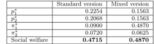
We illustrate our main results summarized in the previous section by the following example. Let the demand function beD(p) = 1−p. We assume that k1= 0.5,k2= 0.4 and in the mixed version of the game firm 1 is the public firm, while firm 2 is the private firm. We calculated the equilibrium prices and payoffs both for the standard version of the game and for the mixed version as well. According to our earlier arguments, we assumed in the example that N E₁ orSP N E₁-type equilibria are played in each case. The following tables show the values calculated for all the three possible orderings of moves.

Table 2 Calculated values for the simultaneous-moves case.

Standard version Mixed version

p^∗₁ 0.2254 0.1563

p^∗₂ 0.2068 0.1563

π₁^∗ 0.0900 0.4870

π₂^∗ 0.0720 0.0625

Social welfare 0.4715 0.4870

Note that in the first column of Table 2 the equilibrium prices, profits and social welfare given for the standard version of the game are expected values as there is no pure-strategy equilibrium in case of simultaneous moves. We have computed these expected values by employing the explicit solution of the Bertrand-Edgeworth game determined by Kreps and Scheinkman (1983).

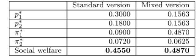
Table 3 Calculated values when firm 1 moves first.

Standard version Mixed version

p^∗₁ 0.3000 0.1563

p^∗₂ 0.3000 0.1563

π₁^∗ 0.0900 0.4870

π₂^∗ 0.1200 0.0625

Social welfare 0.4550 0.4870

The values in Tables 2-4 show the social welfare-increasing effect of the appearance of a public firm, which we emphasized in Section 5.

Table 4 Calculated values when firm 2 moves first.

Standard version Mixed version

p^∗₁ 0.3000 0.1563

p^∗₂ 0.1800 0.1563

π₁^∗ 0.0900 0.4870

π₂^∗ 0.0720 0.0625

Social welfare 0.4550 0.4870

7 Concluding remarks

We analyzed the mixed Bertrand-Edgeworth duopoly game with the following two participants: a private profit-maximizing firm and a public social welfare maximizing firm. We found that the appearance of a public firm is advanta- geous from various points of view. First, the timing of decisions does not play a role since all games with an exogenously given order of moves result in the same outcome. Second, the appearance of a public firm increases social wel- fare. Third, the mixed version of the simultaneous-move Bertrand-Edgeworth game always has an equilibrium in pure strategies.

In our analysis we focused on the interesting case in which the standard Bertrand-Edgeworth game does not have an equilibrium in pure strategies. It should be emphasized that in the other case (i.e.p^c ≥max{p^m₁ , p^m₂}) there is no real difference concerning the market outcome between the standard and mixed versions of the Bertrand-Edgeworth game. In particular, sales take only place at the market clearing price and the entire demand is served at that price regardless of the ordering of moves. However, similarly to the strong private firm case the simultaneous-move game and the private leadership game has an additional implausible outcome of type 3, wheneverk1≤k2 andk1≤D(p^M), in which the private firm sets price p^∗₂ = max

p^M, P(k2) and the public firm a higher price p^∗₁ > max

p^M, P(k₂) . We consider this latter outcome as implausible since this would require that the public firm does not want to enter the market in order achieve at least a positive income or a higher consumer surplus though social welfare remains the same. The equilibria can be determined in an analogous way to the strong private firm case.¹⁷

We have not investigated the situation yet, where more than one private firms exist on the market. However, we should be aware that our knowledge concerning the Bertrand-Edgeworth oligopoly game with only private firms is limited. Even the existence of an equilibrium of multi-period games with exogenously given ordering of moves is not known for the case in which at least pairs of firms move in different time periods. Most recent results on the mixed-strategy equilibria of the simultaneous-move Bertrand-Edgeworth oligopoly game by Hirata (2009) and De Francesco and Salvadori (2010) point to the difficulty of the problem.

17 A detailed proof is available upon request from the authors.

In the current paper we have investigated the production-to-order ver- sion of the Bertrand-Edgeworth game. In a future work we plan to consider the production-in-advance case for which answering the same questions ad- dressed in this paper is much harder. In particular, only the case of symmetric capacities appears to be tractable when comparing the standard production- in-advance price-setting game with its mixed version, since the firms’ mixed- strategy equilibrium profits are only known for that case (see Tasn´adi 2004).

Other questions that could be addressed in future research within the capacity-constrained Bertrand-Edgeworth framework are partial privatization (as initiated by Matsumura 1998), free entry (as investigated for the quantity- setting case, for instance, by Ino and Matsumura 2010), the presence of foreign private firms (see for example, Fjell and Pal 1996), the endogenous emergence of capacity differentials between private and public firms (like by Corneo and Rob 2003 in which the efficiency gap between private and public firms is de- rived from workers’ incentives).

Acknowledgements We are very grateful to two anonymous referees for many helpful comments and suggestions.

References

Anam M, Basher SA, Chiang SH (2007) Mixed oligopoly under demand un- certainty. BE Journal of Theoretical Economics 7:”Article 24”

Anderson SP, de Palma A, Thisse JF (1997) Privatization and efficiency in a differentiated industry. European Economic Review 41:1635–1665

B´arcena-Ruiz JC (2007) Endogenous timing in a mixed duopoly: Price compe- tition. Journal of Economics (Zeitschrift f¨ur National¨okonomie) 91:263–272 Beato P, Mas-Colell A (1984) The marginal cost pricing as a regulation mech- anism in mixed markets. In: Marchand M, Pestieau P, Tulkens H (eds) The Performance of Public Enterprises, North-Holland, Amsterdam, pp 81–100 Boyer M, Moreaux M (1987) Being a leader or a follower: Reflections on the distribution of roles in duopoly. International Journal of Industrial Organi- zation 5:175–192

Corneo G, Jeanne O (1994) Oligopole mixte dans un marche commun. Annales d’Economie et de Statistique 33:73–90

Corneo G, Rob R (2003) Working in public and private firms. Journal of Public Economics 87:1335–1352

Cremer H, Marchand M, Thisse J (1989) The public firm as an instrument for regulating an oligopolistic market. Oxford Economic Papers 41:283–301 Dastidar K, Sinha U (2011) Price competition in a mixed duopoly. In: Dastidar

K, Mukhopadhyay H, Sinha U (eds) Dimensions of Economic Theory and Policy: Essays for Anjan Mukherji, Oxford University Press, New Delhi, p forthcoming

Dastidar KG (1995) On the existence of pure strategy bertrand equilibrium.

Economic Theory 5:19–32

De Francesco M, Salvadori N (2010) Bertrand-edgeworth games under oligopoly with a complete characterization for the triopoly. Munich Per- sonal RePEc Archive, MPRA Paper No 24087

Deneckere R, Kovenock D (1992) Price leadership. Review of Economic Studies 59:143–162

Dowrick S (1986) von stackelberg and cournot duopoly: Choosing roles. Rand Journal of Economics 17:251–260

Fjell K, Pal D (1996) A mixed oligopoly in the presence of foreign private firms. Canadian Journal of Economics 29:737–743

Fraja GD, Delbono F (1989) Alternative strategies of a public enterprise in oligopoly. Oxford Economic Papers 41:302–311

Gal-Or E (1985) First mover and second mover advantages. International Eco- nomic Review 26:649–653

Hamilton J, Slutsky S (1990) Endogenous timing in duopoly games: Stackel- berg or cournot equilibria. Games and Economic Behavior 2:29–46

Harris RG, Wiens EG (1980) Government enterprise: an instrument for the internal regulation of industry. Canadian Journal of Economics 13:125–132 Hirata D (2009) Asymmetric bertrand-edgeworth oligopoly and merg- ers. BE Journal of Theoretical Economics 9:”Article 22”, URL http://www.bepress.com/bejte/topics/art22

Ino H, Matsumura T (2010) What role should public enterprises play in free- entry markets? Journal of Economics (Zeitschrift f¨ur National¨okonomie) 101:213–230

Jacques A (2004) Endogenous timing in a mixed oligopoly: a forgotten equi- librium. Economics Letters 83:147–148

Kreps DM, Scheinkman JA (1983) Quantity precommitment and bertrand competition yield cournot outcomes. Bell Journal of Economics 14:326–337 Levitan R, Shubik M (1972) Price duopoly and capacity constraints. Interna-

tional Economic Review 13:111–122

Lu Y (2007) Endogenous timing in a mixed oligopoly: Another forgotten equi- librium. Economics Letters 94:226–227

Lu Y, Poddar S (2009) Endogenous timing in a mixed duopoly and private duopoly - ‘capacity-then-quantity’ game: The linear demand case. Aus- tralian Economic Papers 48:138–150

Matsumura T (1998) Partial privatization in mixed duopoly. Journal of Public Economics 70:473–483

Matsumura T (2003) Endogenous role in mixed markets: a two production period model. Southern Economic Journal 70:403–413

Ogawa A, Kato K (2006) Price competition in a mixed duopoly. Economics Bulletin 12:1–5

Osborne MJ, Pitchik C (1986) Price competition in a capacity-constrained duopoly. Journal of Economic Theory 38:238–260

Pal D (1998) Endogenous timing in a mixed oligopoly. Economics Letters 61:181–185

Roy Chowdhury P (2009) Mixed duopoly with price competition. Munich Per- sonal RePEc Archive, MPRA Paper No 9220

Tasn´adi A (1999) Existence of pure strategy nash equilibrium in bertrand- edgeworth oligopolies. Economics Letters 63:201–206

Tasn´adi A (2004) Production in advance versus production to order. Journal of Economic Behavior and Organization 54:191–204

Tomaru Y, Kiyono K (2010) Endogenous timing in mixed duopoly with in- creasing marginal costs. Journal of Institutional and Theoretical Economics 166:591–613