Assessing Parkinson’s Disease From Speech Using Fisher Vectors
Jos´e Vicente Egas L´opez
1, Juan Rafael Orozco-Arroyave
2,3, G´abor Gosztolya
1,41
Institute of Informatics, University of Szeged, Szeged, Hungary
2
Faculty of Engineering, University of Antioquia, Medell´ın, Colombia
3
Pattern Recognition Lab, University of Erlangen, Erlangen, Germany
4
MTA-SZTE Research Group on Artificial Intelligence, Szeged, Hungary
egasj @ inf.u-szeged.edu
Abstract
Parkinson’s Disease (PD) is a neuro-degenerative disorder that affects primarily the motor system of the body. Besides other functions, the subject’s speech also deteriorates during the dis- ease, which allows for a non-invasive way of automatic screen- ing. In this study, we represent the utterances of subjects hav- ing PD and those of healthy controls by means of the Fisher Vector approach. This technique is very common in the area of image recognition, where it provides a representation of the local image descriptors via frequency and high order statistics.
In the present work, we used four frame-level feature sets as the input of the FV method, and applied (linear) Support Vec- tor Machines (SVM) for classifying the speech of subjects. We found that our approach offers superior performance compared to classification based on the i-vector and cosine distance ap- proach, and it also provides an efficient combination of machine learning models trained on different feature sets or on different speaker tasks.
Index Terms: Parkinson’s Disease, Fisher Vector encoding, speech analysis, automatic screening
1. Introduction
Shaking, rigidity, slowness of movement, and speech difficul- ties are some of the classic symptoms that affect the motor sys- tem, caused by a decrease of dopamine-producing neurons [1].
Such pathologies are often related to one of the most common neuro-degenerative disorders, that is, Parkinson’s Disease. A person suffering from Parkinson’s is prone to develop changes and disorders in speech and swallowing. This can occur at any time during the disease, but it generally appears as the dis- ease advances. Commonly, the speech of the patient is also affected in terms of its tone, volume, and rate, which leads to dysprosody. Words comprising the speech of the subject may be slurred or mumbled. Additionally, typical articulatory problems exhibited by PD patients are referred to as dysarthia. Also, the speech can fade away at the end of the sentences; likewise, pa- tients may speak slowly and with a breathy kind of speech [1, 2].
Utilizing Computer Tomography (CT) and Magnetic Res- onance Imaging (MRI), the brain scans of people can be har- nessed to diagnose PD. However, their results usually appear to be normal which makes it difficult for physicians to give an ac- curate diagnosis. Currently, there is no existing standard blood or laboratory tests that can be utilized to diagnose PD. Hence, the diagnosis, which sometimes may not be the most accurate, is often made based on the medical history of the patient and/or a neurological examination. In some cases, signs and symptoms of PD may be catalogued as the result of normal aging. Limita- tions within the commonly used process to assess patients with
PD include the high cost and the lack of efficiency when eval- uating the disease. This process generally has two main draw- backs: it greatly depends on the expertise of the clinician, which is subjective; and the limitation of taking the patient to the clinic to try out exhaustive medical assessments and screenings [3].
There is a need to develop quick, reliable and non-invasive ways to diagnose PD. Thus, automatic speech analysis has been utilized in many medical branches in order to tackle the above- mentioned obstacles by offering accurate and non-expensive so- lutions that are able to assess the diagnosis of different neuro- degenerative diseases by the use of speech recordings. The most common scenarios include Alzheimer’s [4, 5, 6] and Parkin- son’s Disease [7, 8], where the performance of different speech processing techniques such as i-vectors or ASR-based features (e.g. speech tempo or hesitation ratio) are applied.
Here, we will utilize the FV approach [9], which is an en- coding method originally developed to represent images as gra- dients of a global generative GMM of low-level image descrip- tors. These new features are fed into a (linear) SVM [10] clas- sifier in order to evaluate their capability to automatically dis- criminate between PD patients and Healthy Controls (HC). We will show that the proposed approach gives a better performance than for instance, using i-vectors, and provides a simple-yet- effective way of combining the predictions with other methods.
To the best of our knowledge, this is the first study that focuses on making use of FV representation in order to detect speech impairments of PD patients.
2. The Fisher Vector approach
The Fisher Vector approach is an image representation that pools local image descriptors (e.g. SIFT, describing occur- rences of rotation- and scale-invariant primitives [11]). In con- trast with the Bag-of-Visual-Words (BoV, [12]) technique, it as- signs a local descriptor to elements in a visual dictionary, ob- tained via a Gaussian Mixture Model for FV. Nevertheless, in- stead of just storing visual word occurrences, these representa- tions take into account the difference between dictionary ele- ments and pooled local features, and they store their statistics.
A nice advantage of the FV representation is that, regardless of the number of local features (i.e. SIFT), it extracts afixed-sized feature representation from each image.
The FV approach has been shown to be quite promising in image representation [9]. Despite the fact that just a handful of studies use FV in speech processing, e.g. for categorizing audio-signals as speech, music and others [13], for speaker ver- ification [14, 15], and for determining the food type from eating sounds [16], we think that FV can be harnessed to improve clas- sification performance in audio processing.
INTERSPEECH 2019
September 15–19, 2019, Graz, Austria
Segmentation
Segmentation
Feature Extraction
Feature Extraction
GMM Training Training
subjects
Test subjects
Fisher Vector encoding
SVM Classification
Fisher Vector encoding Figure 1:Generic methodology applied in our work.
2.1. Fisher Kernel
Named after the statistician Ronald Fisher [9], the Fisher Ker- nel (FK) seeks to measure the similarity of two objects from a parametric generative model of the data (X) which is defined as the gradient of the log-likelihood ofX:
GXλ =5λlogυλ(X), (1) where X = {xt, t = 1, . . . , T} is a sample of T obser- vationsxt ∈ X, υ represents a probability density function that models the generative process of the elements inX and λ = [λ1, . . . , λM]0 ∈ RM stands for the parameter vector υλ[17]. Thus, such a gradient describes the way the parameter υλshould be changed in order to best fit the dataX. A novel way to measure the similarity between two pointsXandY by means of the FK can be expressed as follows [9]:
KF K(X, Y) =GX0λ Fλ−1GYλ. (2) SinceFλis positive semi-definite,Fλ= Fλ−1. Eq. (3) shows how the Cholesky decompositionFλ−1=L0λLλcan be utilized to rewrite the Eq. (2) in terms of the dot product:
KF K(X, Y) =GλX0GλY, (3) where
GλX=LλGXλ =Lλ5λlogυλ(X). (4) Such a normalized gradient vector is the so-calledFisher Vector ofX[17]. Both the FVGλX and the gradient vectorGXλ have the same dimension.
2.2. Fisher Vectors
LetX ={Xt, t= 1. . . T}be the set ofD-dimensional local SIFT descriptors extracted from an image and let the assump- tion of independent samples hold, then Eq. (4) becomes:
GλX=
T
X
t=1
Lλ5λlogυλ(Xt). (5)
The assumption of independence permits the FV to become a sum of normalized gradients statisticsLλ5λlogυλ(xt)calcu- lated for each SIFT descriptor. That is:
Xt→ϕF K(Xt) =Lλ5λlogυλ(Xt), (6) which describes an operation that can be thought of as a higher dimensional space embedding of the local descriptorsXt.
In simple terms, the FV approach extracts low-level local patch descriptors from the audio-signals’ spectrogram. Then,
with the use of a GMM with diagonal covariances we can model the distribution of the extracted features. The log-likelihood gradients of the features modeled by the parameters of such GMM are encoded through the FV [17]. This type of encoding stores the mean and covariance deviation vectors of the compo- nentskthat form the GMM together with the elements of the local feature descriptors. The image is represented by the con- catenation of all the mean and the covariance vectors that gives a final vector of length(2D+ 1)N, forN quantization cells andDdimensional descriptors [17, 18].
The FV approach can be compared with the traditional en- coding method called BoV (Bag of Visual Words), and with a first order encoding method like VLAD (Vector of Locally Aggregated Descriptors). In practice, BoW and VLAD are out- performed by FV due to its second order encoding property of storing additional statistics between codewords and local fea- ture descriptors [19]. Here, we use FV features to encode the MFCC features extracted from audio-signals of HC and PD sub- jects. FV allows us to give a complete representation of the sample set by encoding the count of occurrences and high order statistics associated with its distribution.
3. System description
The architecture designed in our study consists of the follow- ing parts: (1) VAD-based segmentation, (2) feature extraction, (3) fitting a GMM to the local image features, (4) construction of the (audio) word dictionary by means of the GMM, that is, the encoded FV that now represents the global descriptor of the original spectrum, and (5) SVM classification. (See Fig. 1).
3.1. Data
We performed our experiments using the PC-GITA speech cor- pus [20], which contains the recorded speech of 100 Colombian Spanish speakers (50 PD patients and 50 HC). All of the pa- tients were evaluated by a neurologist. The subjects were asked to perform four different tasks during the recordings: six diado- chokinetic (DDK) exercises (e.g. the repetition of the sequence of syllables /pa-ta-ka/), monologue speeches, text reading, and ten short sentences.
3.2. Feature Extraction
Following the study of [21], we performed our experiments us- ing four different feature sets. The first consisted of 20 MFCCs, obtained from 30 ms wide windows; and the rest of the feature sets were built by articulation, phonation, and prosody, respec- tively. Before extracting the features we performed speech/non- speech segmentation by means of Voice Activity Detection
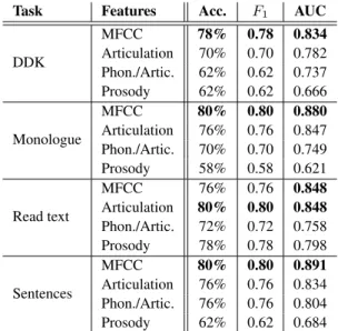
Table 1:Results obtained for the various tasks and feature sets
Task Features Acc. F1 AUC
DDK
MFCC 78% 0.78 0.834
Articulation 70% 0.70 0.782 Phon./Artic. 62% 0.62 0.737
Prosody 62% 0.62 0.666
Monologue
MFCC 80% 0.80 0.880
Articulation 76% 0.76 0.847 Phon./Artic. 70% 0.70 0.749
Prosody 58% 0.58 0.621
Read text
MFCC 76% 0.76 0.848
Articulation 80% 0.80 0.848 Phon./Artic. 72% 0.72 0.758
Prosody 78% 0.78 0.798
Sentences
MFCC 80% 0.80 0.891
Articulation 76% 0.76 0.834 Phon./Artic. 76% 0.76 0.804
Prosody 62% 0.62 0.684
(VAD), and also by voiced/unvoiced using the auto-correlation method from Praat [22]. For articulation evaluation, the first 22 Bark bands (BBE) invoiced/unvoicedandunvoiced/voiced transitions were treated as features [23]. Features obtained from phonation and articulation invoiced segmentsconstitute a 14- dimensional vector with 30 ms of windows analysis and 5 ms of time shift. These features contained log-energy, pitch (F0), first and second formants (F1,F2) together with their first and second derivatives, Jitter and Shimmer. Prosody information was represented by means of the approach introduced in [24];
hence, we got a 13-dimensional feature vector formed by us- ing the number of voiced frames per segment and the 12 coef- ficients. To construct the FV representation, we experimented withN= 2,4,8,16,32,64and128Gaussian components. We utilized the VLFeat library in order to get the fisher vectors [25].
3.3. Classification
SVM was utilized to classify audio-signals into the PD and HC class labels. SVM was found to be robust even with a large number of dimensions and it was shown to be efficient when used with FV [17, 26] due to it being a discriminative classifier that provides a flexible decision boundary. We used the libSVM implementation [27] with a linear kernel, as suggested in [9];
theCcomplexity parameter was set in the range10−5,. . .,101. The PC-GITA dataset is not large enough to define sepa- rate train, development and test sets; so in order to avoid any form of peeking, we performed the experiments in a speaker- independent 10-foldnested cross-validation(CV) setting; each fold contained the utterances of 5 PD and 5 HC speakers. Clas- sification was made by using the SVM model trained on 9 folds (i.e. 90 speakers) and to get the right meta-parameters, we per- formedanother CVover the 90 speakers of the training folds.
After determining the optimalN(number of Gaussian compo- nents for FV) andC(SVM complexity) meta-parameters, we trained a SVM model with the 90 speakers using these meta- parameter values. This way, we obtained predictions for all speakers without relying on any kind of data or information about the given subject.
Figure 2:Achieved AUC values as a function ofNfor the four speaker tasks, when using the MFCC feature set.
3.4. Evaluation
The decisions made by the SVM were used to calculate the Area Under the Receiver Operating Characteristics Curve (AUC), which is a widely used statistic for summarizing the perfor- mance of automatic classification systems in medical applica- tions. In addition, we calculated the classification accuracy and F-measure (orF1) scores. These metrics were calculated by choosing the decision threshold along with the Equal Error Rate (EER). Since the class distribution was balanced, classification accuracy andF1score were identical in each case. During the nested cross-validation procedure we determined the optimal meta-parameters as those that led to the highest AUC value.
4. Results
Table 1 lists the results we obtained for the different speaker tasks and the different frame-level feature sets, the best values for a given task being shown inbold. We observe that the best scores in each case were gotten with the MFCC feature set (ex- cept for the ‘Read text’ task, where the accuracy andF1-scores appeared to be higher with articulatory features along with an identical AUC score). Although this was the case in our earlier studies as well (see [21]), where we relied on i-vectors, now the difference is significantly larger. This is probably because the FV approach assumed that the frame-level feature values could be modeled along with a diagonal covariance matrix. This as- sumption is quite realistic for MFCCs and, perhaps, for the filter bank values, of the voiced/unvoiced transitions (i.e. the articu- latory features), but it may not be true for the phonational and prosodic attributes.
In the next experiment, we focused on the trends in the op- timal number of Gaussian components (i.e. N) for the tasks.
We tried out all the possibleNvalues, and then just theCcom- plexity parameter was determined in a nested CV. (Of course, this was not a completely fair setup from a machine learning perspective. Still, in our opinion, this small amount of ‘peek- ing’ was both necessary and acceptable in this scenario. Then we could focus on classification performance as a function of N.) Fig. 2 shows the AUC scores for the MFCC features. In general, using fewer GMMs (N≤16) led to a sub-optimal per- formance, excepting the DDK task, where we can see a close-to- optimal AUC value even forN = 16. For the Monologue task, N = 32components were needed for optimal performance, whileN= 64andN= 128were enough for the Read text and the Sentences tasks, respectively. AUC scores were above 0.8
Table 2:Results obtained when combining the different feature sets for the ‘Monologue’ task
Features Acc. F1 AUC
MFCC 80% 0.80 0.880
MFCC + Articulation 84% 0.84 0.908
MFCC + Phon./Artic. 78% 0.78 0.871
MFCC + Prosody 78% 0.78 0.878
MFCC + Artic. + Phon./Artic 82% 0.82 0.897 MFCC + Artic. + Prosody 84% 0.84 0.900
All feature sets 82% 0.82 0.895
for three tasks even forN = 4; as it meant 104-176 attributes for each subject, we achieved relatively high classification per- formance even with this compact representation.
5. Classifier Combination
For i-vectors the straightforward ‘classification’ approach is to compare the i-vector of the test speaker with the reference i- vector by taking the cosine distance. This approach has a solid mathematical basis and it tends to perform well in practice but it makes the predictions hard to combine with other methods or feature sets. Here, we used a standard SVM, which generates class-wise posterior estimates that provide a simple way of clas- sifier combination by taking the mean of two or more posterior vectors (late fusion[28]).
We will demonstrate the effectiveness of this strategy with two short examples. Instead of applying more classification al- gorithms, we will focus on combining the differentfeature sets and tasks. We will apply late fusion by taking the weighted mean of the posterior estimates with an increment of 0.05;
and similar to our earlier experiments, weights are determined in a nested cross-validation process. We choose the feature sets or tasks by applying the Sequential Forward Selection (SFS, [29, 30]) approach. First we start with the feature set/task that has the highest metric value. Then we try adding all the remaining feature sets/tasks one by one, and select the one that leads to the highest improvement in the AUC score. Values ex- ceeding the initial feature set/task are shown inbold.
5.1. Results with Feature Set Combination
Table 2 shows the results obtained for the Monologue task. Note that the results regarding the MFCC feature set improve when articulatory features are added: the classification accuracy rose from 80% to 84%, the correspondingF1value went up from 0.8 to 0.84, and the AUC value of the PD class also rose from 0.880 to 0.908. However, adding more feature sets proved futile: al- though the accuracy and F-measure values remained constant even after utilizing the prosodic features as well, the AUC score fell to 0.900. Still, the 0.908 score achieved by fusing the pre- dictions got from the first two feature sets brought an improve- ment of 20% in terms of the RER.
5.2. Results with Task Set Combination
Table 3 lists the accuracy, F-measure and AUC scores we ob- tained when combining the posterior estimates for the different speech tasks besides articulatory features. We got the highest results on the ‘Read text’ task. It actually matched the perfor- mance of MFCCs in terms of the AUC, while the accuracy and F1 values appeared to be higher. Besides ‘Read text’, using
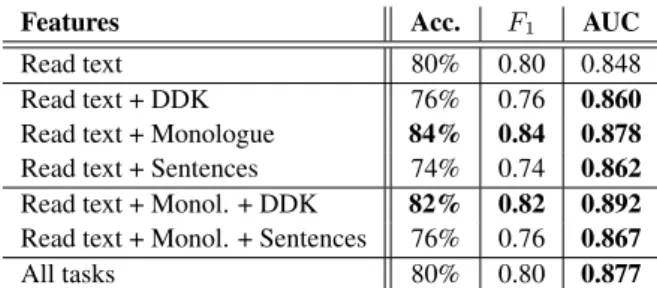
Table 3: Results obtained when combining the different tasks for the articulatory features
Features Acc. F1 AUC
Read text 80% 0.80 0.848
Read text + DDK 76% 0.76 0.860
Read text + Monologue 84% 0.84 0.878 Read text + Sentences 74% 0.74 0.862 Read text + Monol. + DDK 82% 0.82 0.892 Read text + Monol. + Sentences 76% 0.76 0.867
All tasks 80% 0.80 0.877
the ‘Monologue’ task resulted in a performance improvement, while incorporating the ‘DDK’ task as well increased the AUC value even further (although the classification accuracy andF1
dropped slightly), leading to a 29% of RER score.
Overall, we achieved significant improvements in both cases by training SVMs for the task-feature set pairs indepen- dently, and taking the weighted mean of the posterior estimates.
The combination of weights were determined in nested cross- validation, so it was free of peeking. Our results indeed confirm the flexibility of FV representations. For state-of-the-art perfor- mance, it might worth combining different classifiers as well.
6. Conclusions
Parkinson’s Disease, a chronic neuro-degenerative disease, is often difficult to diagnose accurately. A non-invasive and promising procedure for assessing and diagnosing Parkinson’s is the automatic analysis of speech of the subject. Our study showed how useful are FV over i-vectors as features in the as- sessment of PD via the analysis of speech. We used the PC- GITA dataset to classify PD and HC subjects. Samples com- prising such dataset were segmented, and cepstral, articulatory, phonological and prosodic features were extracted from the voiced parts. These features were represented by FV-encoding and were classified using Support-Vector Machines. This work- flow produced a high-precision classification performance.
The first experiments revealed that MFCC features per- formed the best in three of the four tasks. The task ’Sen- tences’ became the leader in terms of the AUC, with a score of 0.891. In the subsequent experiments, we showed that the predictions obtained for the different frame-level feature sets and tasks could be combined, allowing an even higher classifi- cation performance. This way, our AUC scores improved even further, and we got 0.908 with the combination of MFCCs with articulatory features for the ’Monologue’ task, while using the articulatory features, but incorporating the predictions for the tasks ‘Read text’, ‘Monologue’ and ‘DDK’, also led to a sig- nificant improvement over relying on the ’Read text’ task only.
Using different feature sets and/or tasks is not the only possible combination approach possible. Another promising line of re- search is to apply other machine learning methods, and combine their predictions. This, however, is the subject of future works.
7. Acknowledgements
This research was partially funded by the Ministry of Human Capacities, Hungary (grant 20391-3/2018/FEKUSTRAT). This work was also funded by COD at UdeA grant # PRG2015-7683.
G. Gosztolya was also funded by the J´anos Bolyai Scholarship of the Hungarian Academy of Sciences.
8. References
[1] L. V. Kalia and A. E. Lang, “Parkinon’s disease,”The Lancet, vol.
386, no. 4, pp. 896–912, 2015.
[2] S. Pinto, R. Cardoso, J. Sadat, I. Guimar˜aes, C. Mercier, H. San- tos, C. Atkinson-Clement, J. Carvalho, P. Welby, P. Oliveiraet al.,
“Dysarthria in individuals with Parkinson’s disease: a protocol for a binational, cross-sectional, case-controlled study in French and European Portuguese (fralusopark),”BMJ open, vol. 6, no. 11, p.
e012885, 2016.
[3] D. G. Theodoros, G. Constantinescu, T. G. Russell, E. C. Ward, S. J. Wilson, and R. Wootton, “Treating the speech disorder in Parkinon’s disease online,”Journal of Telemedicine and Telecare, vol. 12, no. 3 suppl, pp. 88–91, 2006.
[4] A. Satt, R. Hoory, A. K¨onig, P. Aalten, and P. H. Robert, “Speech- based automatic and robust detection of very early dementia,” in Proceedings of Interspeech, Singapore, 2014, pp. 2538–2542.
[5] M. Shahbakhi, D. T. Far, E. Tahamiet al., “Speech analysis for diagnosis of Parkinson’s disease using genetic algorithm and sup- port vector machine,”Journal of Biomedical Science and Engi- neering, vol. 7, no. 4, pp. 147–156, 2014.
[6] G. Gosztolya, V. Vincze, L. T´oth, M. P´ak´aski, J. K´alm´an, and I. Hoffmann, “Identifying Mild Cognitive Impairment and mild Alzheimers disease based on spontaneous speech using ASR and linguistic features,”Computer, Speech & Language, vol. 53, no.
Jan, pp. 181–197, 2019.
[7] L. Zhou, K. C. Fraser, and F. Rudzicz, “Speech recognition in Alzheimer’s disease and in its assessment.” inINTERSPEECH, 2016, pp. 1948–1952.
[8] L. Moro-Vel´azquez, J. A. G´omez-Garc´ıa, J. I. Godino-Llorente, J. Villalba, J. R. Orozco-Arroyave, and N. Dehak, “Analysis of speaker recognition methodologies and the influence of kinetic changes to automatically detect Parkinon’s disease,”Applied Soft Computing, vol. 62, pp. 649–666, 2018.
[9] T. S. Jaakkola and D. Haussler, “Exploiting generative models in discriminative classifiers,” inProceedings of NIPS, Denver, CO, USA, 1998, pp. 487–493.
[10] B. Sch¨olkopf, J. C. Platt, J. Shawe-Taylor, A. J. Smola, and R. C.
Williamson, “Estimating the support of a high-dimensional dis- tribution,”Neural Computation, vol. 13, no. 7, pp. 1443–1471, 2001.
[11] D. G. Lowe, “Distinctive image features from scale-invariant key- points,”International Journal of Computer Vision, vol. 60, no. 2, pp. 91–110, 2004.
[12] X. Peng, L. Wang, X. Wang, and Y. Qiao, “Bag of visual words and fusion methods for action recognition: Comprehensive study and good practice,”Computer Vision and Image Understanding, vol. 150, pp. 109–125, 2016.
[13] P. J. Moreno and R. Rifkin, “Using the Fisher kernel method for web audio classification,” inProceedings of ICASSP, Dallas, TX, USA, 2010, pp. 2417–2420.
[14] Y. Tian, L. He, Z. yi Li, W. lan Wu, W.-Q. Zhang, and J. Liu,
“Speaker verification using Fisher vector,” inProceedings of ISC- SLP, Singapore, Singapore, 2014, pp. 419–422.
[15] Z. Zaj´ıc and M. Hr´uz, “Fisher Vectors in PLDA speaker verifica- tion system,” inProceedings of ICSP, Chengdu, China, 2016, pp.
1338–1341.
[16] H. Kaya, A. A. Karpov, and A. A. Salah, “Fisher Vectors with cascaded normalization for paralinguistic analysis,” inProceed- ings of Interspeech, 2015, pp. 909–913.
[17] J. S´anchez, F. Perronnin, T. Mensink, and J. Verbeek, “Image clas- sification with the Fisher Vector: Theory and practice,”Interna- tional Journal of Computer Vision, vol. 105, no. 3, pp. 222–245, 2013.
[18] F. Perronnin and C. Dance, “Fisher kernels on visual vocabularies for image categorization,” in2007 IEEE Conference on Computer Vision and Pattern Recognition, June 2007, pp. 1–8.
[19] M. Seeland, M. Rzanny, N. Alaqraa, J. W¨aldchen, and P. M¨ader, “Plant species classification using flower images:
A comparative study of local feature representations,” PLOS ONE, vol. 12, no. 2, pp. 1–29, 02 2017. [Online]. Available:
https://doi.org/10.1371/journal.pone.0170629
[20] J. R. Orozco-Arroyave, J. D. Arias-Londo˜no, J. F. Vargas-Bonilla, M. C. Gonzalez-R´ativa, and E. N¨oth, “New Spanish speech cor- pus database for the analysis of people suffering from Parkinson’s Disease,” inProceedings of LREC, Reykjavik, Iceland, May 2014, pp. 26–31.
[21] N. Garc´ıa, J. R. Orozco-Arroyave, L. F. D’Haro, N. Dehak, and E. N¨oth, “Evaluation of the neurological state of people with Parkinon’s disease using i-vectors,” inINTERSPEECH, 2017.
[22] P. Boersma, “Accurate short-term analysis of the fundamental fre- quency and the harmonics-to-noise ratio of a sampled sound,” in IFA Proceedings 17, 1993, pp. 97–110.
[23] J. R. Orozco-Arroyave, J. V´asquez-Correa, F. H¨onig, J. D. Arias- Londo˜no, J. Vargas-Bonilla, S. Skodda, J. Rusz, and E. N¨oth, “To- wards an automatic monitoring of the neurological state of Parki- non’s patients from speech,” inProceedings of ICASSP. IEEE, 2016, pp. 6490–6494.
[24] N. Dehak, P. Dumouchel, and P. Kenny, “Modeling prosodic features with joint factor analysis for speaker verification,”
IEEE Transactions on Audio, Speech, and Language Processing, vol. 15, no. 7, pp. 2095–2103, 2007.
[25] A. Vedaldi and B. Fulkerson, “Vlfeat: An open and portable li- brary of computer vision algorithms,” inProceedings of the 18th ACM international conference on Multimedia. ACM, 2010, pp.
1469–1472.
[26] D. C. Smith and K. A. Kornelson, “A comparison of Fisher vectors and Gaussian supervectors for document versus non-document image classification,” inApplications of Digital Image Processing XXXVI, vol. 8856. International Society for Optics and Photon- ics, 2013, p. 88560N.
[27] C.-C. Chang and C.-J. Lin, “LIBSVM: A library for support vector machines,”ACM Transactions on Intelligent Systems and Technology, vol. 2, pp. 1–27, 2011.
[28] B. Schuller, S. Steidl, A. Batliner, S. Hantke, E. Bergelson, J. Kra- jewski, C. Janott, A. Amatuni, M. Casillas, A. Seidl, M. Soder- strom, A. S. Warlaumont, G. Hidalgo, S. Schnieder, C. Heiser, W. Hohenhorst, M. Herzog, M. Schmitt, K. Qian, Y. Zhang, G. Trigeorgis, P. Tzirakis, and S. Zafeiriou, “The INTERSPEECH 2017 computational paralinguistics challenge: Addressee, Cold
& Snoring,” inProceedings of Interspeech, Stockholm, Sweden, Aug 2017, pp. 3442–3446.
[29] M. Last, A. Kandel, and O. Maimon, “Information-theoretic algo- rithm for feature selection,”Pattern Recognition Letters, vol. 22, no. 6-7, pp. 799–811, 2001.
[30] I. A. Basheer and M. Hajmeer, “Artificial neural networks: funda- mentals, computing, design, and application,”Journal of microbi- ological methods, vol. 43, no. 1, pp. 3–31, 2000.