Probabilistic Sampling DNN Training

(1)

TEX CLASS FILES, VOL. 14, NO. 8, AUGUST 2015

Social Signal Detection by

Probabilistic Sampling DNN Training

G ábor Gosztolya, Tam ás Gr ósz, and L ászl ó T óth,Member, IEEE

Abstract—When our task is to detect social signals such as laughter and filler events in an audio recording, the most straightforward way is to apply a Hidden Markov Model – or a Hidden Markov Model/Deep Neural Network (HMM/DNN) hybrid, which is considered state-of-the-art nowadays. In this hybrid model, the DNN component is trained on frame-level samples of the classes we are looking for. In such event detection tasks, however, the training labels are seriously imbalanced, as typically only a small fraction of the training data corresponds to these social signals, while the bulk of the utterances consists of speech segments or silence. A strong imbalance of the training classes is known to cause difficulties during DNN training. To alleviate these problems, here we apply the technique called probabilistic sampling, which seeks to balance the class distribution. Probabilistic sampling is a mathematically well-founded combination of upsampling and downsampling, which was found to outperform both of these simple resampling approaches. With this strategy, we managed to achieve a 7–8% relative error reduction both at the segment level and frame level, and we efficiently reduced the DNN training times as well.

Index Terms—Deep neural networks, instance sampling, social signals, laughter detection.

✦

1 INTRODUCTION

W

^ITHIN speech technology, an emerging area is pa- ralinguistic phenomenon detection, which seeks to locate non-linguistic events (conflict, laughter events, etc.) in speech. One task belonging to this area is the detection of social signals, from which perhaps laughter and filler events (vocalizations like “um”, “eh”, “er” etc.) are the most important. Many experiments were performed with the goal of detecting laughter (e.g. [1], [2], [3]), and the detection of filler events has also become popular recently (e.g. [4], [5], [6], [7], [8], [9]).

Most of the earlier studies focused on the frame level (e.g. [5], [10], [11]). However, a more realistic approach is to detect occurrences of the given phenomena. To do this, one may simply borrow techniques from Auto- matic Speech Recognition (ASR), such as applying a Hid- den Markov Model (HMM) to combine the local (frame- level) likelihood estimates of a Gaussian Mixture Model (GMM) into segment-level occurrence hypotheses. Nowa- days in ASR, with the invention of Deep Neural Networks (DNNs), HMM/GMMs have been replaced by the so-called HMM/DNN hybrids as state-of-the-art [12], and this technique may be readily applied in this task as well.

To construct a HMM/DNN-based event detector, we train our DNNs on frame-level samples of the classes we are looking for (e.g. laughter) and background events (e.g.

speech, silence, background noise). However, social signals are relatively rare phenomena in spontaneous speech, typically taking up only a small fraction of speech time [13].

This means that we have to train our DNNs on a data

• G. Gosztolya and L. T´oth are with the MTA-SZTE Research Group on Artificial Intelligence of the Hungarian Academy of Sciences and the University of Szeged, Hungary.

E-mail:{ggabor, tothl}@ inf.u-szeged.hu

• T. Gr´osz is with the University of Szeged, Hungary.

E-mail: groszt@inf.u-szeged.hu

Manuscript received April 19, 2005; revised August 26, 2015.

set where the distribution of examples belonging to the different classes are heavily imbalanced. Neural networks are known to be sensitive to (a strong) class imbalance (see e.g. [14]), and DNNs are no exception. Fortunately, in ASR the distribution of the phones are not so imbalanced that it would cause noticeable training difficulties. Also, we usually apply context-dependent state tying (see e.g. [15], [16], [17]), which also tends to reduce the difference in the number of examples belonging to the different states (i.e.

classes). However, in the case of social signal detection the imbalance of the classes is much more dramatic, and it needs to be handled carefully.

The simplest solution to help balance the distribution of training samples associated with the different classes is to re-sample the input data. In its simplest form it means that we simply discard training data from the more frequent classes (filtering or down-sampling approach [18]), which clearly decreases the variability of the training data, and this may result in a loss of accuracy.

Of course, re-sampling is not the only way to balance the class distribution of the training data. Another choice, being very popular in image processing, is that of data augmentation; that is, generating further training examples from the existing ones. In image processing, this typically means rotating, mirroring and resizing images, and changes in the colours [19], [20], [21]. In ASR, some studies suggest that speeding up or slowing down utterances slightly [22], adding noise to the speech signal [23] or utilizing vocal tract length perturbation [24], [25] are useful methods to increase the size of training sets in low-resource scenarios.

Notice, however, that while generating new images can easily be applied for balancing class distribution, in speech processing, where each utterance tends to contain thousands of training examples associated with several classes, it is not so straightforward to realize. The ASR studies listed above all focused on creating more training examples in general,

(2)

and not just for specific classes.

The data augmentation approaches mentioned so far all operate before feature extraction, i.e. they create “new”

images or speech recordings. Another type of data augmentation methods operate in the “feature space” instead of this “data space”: they create synthetic examples based on thefeature vectorsof existing training examples. Perhaps the most popular such algorithm is the Synthetic Minority Over-sampling Technique (SMOTE, [26]), which takes the linear combination ofk nearest neighbours of a randomly chosen example in the feature space.

These methods, despite being more task-independent than the former ones, appear to be quite hard to apply in ASR (or in the detection of laughter or filler events). The reason for this is that it is common practice to train the acoustic DNNs on a sliding window of feature vectors to improve performance. As the consecutive feature vectors of an utterance are typically stored after each other in the memory, using the feature vectors of the neighbouring frames imposes no additional memory requirement. However, if we generate further synthetic examples via SMOTE (or some similar method), we have to handle the neighbouring feature vectors as well. If we leave them as they are, our newly generated examples will differ from the original ones only in a fraction of their feature values. However, to use SMOTE for generating new feature values for the “neighbouring”

frames as well would expand our memory requirements (e.g. using 7 frames at each side leads us to use 15 times as much memory), since the generated “neighbours” cannot be re-used for other training examples.

For these reasons, in this study, to detect laughter and filler events in English mobile phone conversations, we will not apply data augmentation, but focus on training data re-sampling. Instead of the simple approaches of down- and upsampling (i.e. use the examples of the rarer classes less and more frequently, respectively), we will utilize a more sophisticated technique called probabilistic sampling, which is a mathematically well-founded combination of the two approaches. We will also present an efficient way of implementing this sampling strategy, which meets the needs of speech processing.

The structure of this paper is as follows. First, we will introduce probabilistic sampling, give an implementation approach which efficiently reduces the randomness present during DNN training, and discuss how applying probabilistic sampling affects the application of DNNs in Hidden Markov Models. Then we will describe the experimental set- up: the database used, the DNN parameters, the language model used, explain the way the meta-parameters were fine- tuned, and discuss the evaluation metrics used. Afterwards we will present and analyze our results, where besides event detection accuracy, we examine how the application of probabilistic sampling affected the training times of our DNN-based acoustic models, and also look at how the output likelihood values changed.

2 PROBABILISTIC SAMPLING

Like most machine learning algorithms, neural nets are sensitive to class imbalances, and tend to behave inaccurately

on classes having only a few examples. The simplest solution to help balance the class distribution is to downsample the more frequent classes, but it results in data loss, and hence may also result in a drop in accuracy. A more refined solution is to upsamplethe rarer classes: we utilize the examples from these classes more frequently during training.

A mathematically well-formulated re-sampling strategy is the training scheme called probabilistic sampling [27], [28].

This procedure selects the next training sample following a two-step sampling scheme: first we select a class according to some probability distribution, then we randomly pick a training sample that belongs to this class. For the first step, we assign the following probability to each class:

P(c^k) =λ1

K + (1−λ)P rior(c^k), (1) whereP rior(ck)is the prior probability of classck, K is the number of classes andλ ∈ [0,1]is a parameter. For λ = 0, the above formula returns the original class distribution, so probabilistic sampling will behave just as conventional sampling does. For λ = 1, we get a uniform distribution over the classes, so we get totally balanced samples with respect to class frequency. Selecting aλvalue between 0 and 1 allows us to interpolate between the two distributions.

(For the sake of simplicity, for each iteration we select the same number of samples as there are in the training set.)

Database sampling is quite rarely applied either in ASR or in similar areas. We should mention the in-depth study of Garc´ıa-Moral et al. [29], who discarded examples belonging to the more common classes. Although this made the ANN training process much faster, they also experienced a slight drop in accuracy. T ´oth and Kocsor applied this probabilistic sampling approach to a very small speech recognition task in 2005 [28], and they were able to improve the recognition accuracy. More recently, Gr´osz et al. applied probabilistic sampling in the training of DNN acoustic models with context-dependent targets. With this strategy they obtained significant reductions in the word error rate in two large- vocabulary speech recognition tasks [30]. These studies focused on speech recognition, where the class imbalance is relatively small; still the probabilistic sampling technique resulted in performance gains. When the task is social signal detection, where the class imbalance is usually much larger, we can reasonably expect that applying this technique will result in significant improvements in the scores.

2.1 Efficient Implementation for Speech Processing Notice that the basic version of the probabilistic sampling scheme introduces randomness in the sampling process at two distinct points: first we randomlypick a class, and then werandomlypick a training sample of the given class.

Although usually we have millions of training frames, for some events of interest the number of training examples is much more limited. If we follow this scheme, it may happen that some examples are not used at all during training.

In standard ANN training, the typical data random- ization process consists of shuffling the data vectors in a random order before training. This process guarantees that all the training samples get processed. This gave us the idea of implementing probabilistic sampling as follows.

(3)

TEX CLASS FILES, VOL. 14, NO. 8, AUGUST 2015 t1 t

2 t

3 t

4 t

5 t

6 t

7 t

8 t

9 t

10 t

11 t

12 t

13 t

14 t

15 t

16 t

17 t

18 t

19 t

20 t

21 t

22 t

23 t

24 t

25

. . . . . .

Feature vectors (i.e. MFCC or FBANK)

Class label pointers

c1

. . .

c2

. . .

c3

. . .

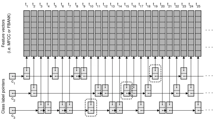
Fig. 1. The basic scheme of the proposed probabilistic sampling implementation approach. The pointers to the frame-level feature vectors are stored in a linked list data structure separately for each class, allowing the efficient location of the next training sample of each class and easy access to the neighbouring frame-level feature vectors. The dashed circles show the pointers to the next training instance for each class employed during training.

In our approach, first we set up separate linked list data structures [31] for each class. These linked lists store pointers to each frame-level feature vector associated with the given class (see Figure 1). Then we shuffle the nodes of each linked list (i.e. the training examples). Before starting the first training iteration, we also set pointers to the first example ofeach class.

During training, first we randomly select a class, following the multinomial distribution of Eq. (1). Then, however, instead of randomly picking a sample within the class, we use the training sample (i.e. frame) indicated by the pointer of the given class, and advance the pointer to the next sample. (If this was the last sample of the actual class, we set our pointer to the first one.) This way we can guarantee that, for each class, all of its training samples will be used with roughly the same frequency, avoiding the possibility of not using or underusing certain samples. Notice that with this approach we need only two pointers for each example (one pointing to the address of the actual feature vector, and one referring to the next node of the linked list), which is negligible, compared to the size of the training data.

Another important aspect of various frame-level speech tasks is that nowadays it is standard practice to train frame-level classifiers on a sliding windowof neighbouring frames instead of using only the feature vector of a single frame. That is, instead of using the xt observation vector associated with the tth frame, we use the 2k + 1-frame long xt−k, . . . , xt, . . . , xt+k concatenated feature vector to classify the tth frame. If we had opted for simply sorting the feature vectors by their class labels, we would have had to store the feature values belonging to the neighbouring frames as well, which would multiply the memory require-

ments of DNN training. However, by storing only a pointer referring to the location of the feature vector of the given frame, we can easily access the feature vectors of both the preceding and the subsequent neighbouring frames.

2.2 Application in a HMM/ANN Hybrid

A standard Hidden Markov Model requires frame-level estimates of the class-conditional likelihoodp(x^t|c^k)for the given observation vectorxt, which are provided by a gen- erative method like Gaussian Mixture Models (GMMs) [32].

When we replace GMMs by neural networks, which estimate P(c^k|x^t), the p(x^t|c^k) values expected by the HMM can be got using Bayes’ theorem. So, in a HMM/ANN hybrid, we divide the posterior estimates produced by the ANN (or DNN) by the priors of the classes, i.e. by P rior(ck). This will give the required likelihood values within a scaling factor, which can be ignored as it has no influence on the subsequent search process.

In contrast, T ´oth and Kocsor showed that when we train the neural network using a uniform class distribution (being equivalent to using probabilistic sampling with λ = 1), the networks will estimate directly the class-conditional p(x^t|c^k)values within a scaling factor [28]. This means that when we integrate our classifiers trained with λ = 1into a HMM/ANN hybrid, we should omit the division of the network outputs by the class priors.

Theoretically we should either use λ = 0 and divide by the class priors, or use λ = 1 and not divide by the priors. However, in practice the probability estimates are not precise. While with standard sampling (λ = 0) ANNs tend to underestimate the probability of the rarer classes, chances are that they will be overestimated in the case of

(4)

TABLE 1

The distribution of laughter and filler events in the SSPNet Vocalization Corpus

Total Count Total Duration (sec) Total Duration (%)

Set Utterances Laughter Fillers Utterances Laughter Fillers Laughter Fillers

Training 1583 649 1710 17358 593 850 3.4% 4.9%

Development 500 225 556 5478 258 294 4.7% 5.4%

Test 680 284 722 7444 240 355 3.2% 4.8%

Total 2763 1158 2988 30280 1091 1499 3.6% 5.0%

uniform sampling (λ = 1). T ´oth and Kocsor [28] achieved the best performance withλvalues strictly between 0 and 1, and we also recommend finding the best value for the given task experimentally.

In this study we propose another likelihood normaliza- tion strategy. The explanation presented in [28] tells us why (theoretically) we have to divide the output likelihoods by the original class priors when we train DNNs withλ = 0, and why we should avoid any division in the case ofλ= 1.

Experimentally, however, intermediateλvalues were found to be optimal. With these intermediateλvalues, actually a thirdclass distribution is used during training. This means that we should in fact divide the output likelihood estimates of a DNN by the prior probabilities of the classes given by the P(c^k) values calculated using Eq. (1). As the third option, we also tested this approach for both λ = 0 and λ= 1, as well as for intermediateλvalues.

3 EXPERIMENTAL SETUP

3.1 The SSPNet Vocalization Corpus

We performed our experiments on the SSPNet Vocaliza- tion Corpus [4], which consists of 2763 short audio clips extracted from telephone conversations, containing 2988 laughter and 1158 filler events (see Table 1). In this corpus just3.6%of the duration corresponds to laughter, and5.0%

consists of filler events; the remaining 91.6% consists of miscellaneous speech (51.2%) and silence (40.2%). Unfor- tunately, in the public annotation only the laughter and filler events are marked, so in our experiments each frame was labeled as one of three classes: “laughter”, “filler”

or “garbage” (meaning both silence and non-filler non- laughter speech). We will follow the standard split of the dataset into a training, development and test set, introduced at the Interspeech Computational Paralinguistics Challenge (ComParE) in 2013 [10]. From the total of 2763 clips, 1583 were assigned to the training set, 500 clips to the development set, and 680 clips to the test set.

3.2 Evaluation Metrics

For tasks like social signal detection, where the distribution of classes is significantly biased, classification accuracy is only of limited use. Also, although on this dataset and in social signal detection in general it is common to rely on the Area-Under-the-Curve (AUC) score of the frame- level posteriors for the classes of interest (now laughter and filler events) (e.g. [5], [10], [33], [34]), it was shown recently (see [35]) that frame-level AUC is an unreliable metric for this task. Besides raising several theoretical objections,

Gosztolya showed experimentally that the AUC values can be significantly improved by applying a simple smoothing over time on the output likelihoods (a technique applied in several studies, e.g. [5], [11], [33], [34], [36], [37]), but this transformation makes the scores unsuitable for a Hidden Markov Model.

Because of this, we decided to apply a HMM to perform event occurrence detection, and calculated accuracy metrics based on these occurrences. We applied the standard infor- mation retrieval metrics of precision, recall and F-measure (or F1-score) [38]. We combined the scores of the two social signals by macro-averaging: we averaged the precision and recall scores of the two phenomena in an unweighted manner, and calculatedF1from these average values.

Another open question is how we should calculate the number of true positives, false positives and false nega- tives. One way to do this is that, after applying the Hidden Markov Model, we compare the resulting event occurrence hypotheses with the manual annotation frame-by-frame.

This approach was followed by e.g. Salamin et al. [4]. There are similar evaluation approaches available for the task of speaker diarization as well (see e.g. [39], [40]).

However, frames are in fact an intermediate step required only for technical reasons, and they are used relatively rarely in actual evaluations. In ASR only the phoneme (word) sequence recognized is compared with the ground truth transcript, and the time-alignment is completely ignored. The reason for this is partly that it is impossible to objectively position phoneme boundaries within a 10ms precision, which is the typical frame-shift: due to the continuous movement of the vocal chords and the mouth, we can expect no clear-cut boundary between two consecutive phonemes. Even from the aspect of user expectations, lo- cating an event occurrence with slight differences at the starting and ending positions still obviously counts as a perfect match. The requirement of frame-level precision is avoided if we rate the performance at the segment level, where slight differences in time alignment are tolerated.

To decide whether two occurrences of events (i.e. a laughter occurrence hypothesis returned by the HMM and one labelled by a human annotator) match, there is no de facto standard in the literature. For example, Gosztolya required only that the two occurrences refer to the same kind of event (i.e. in our case laughter or filler) and that their time intervals intersect [35]. Pokorny et al. [41] also matched the occurrences by checking whether their time intervals intersected, allowing several event occurrence hypotheses to match one manually annotated occurrence. In the NIST standard for Spoken Term Detection evaluation [42], the centre of the two occurrences have to fall close to each other

(5)

(i.e. within a threshold). In this study we combined the two approaches: we required that the two occurrences intersect, while their centre also had to be close to each other (within 500ms, as in the NIST STD standard [42]).

We performed our experiments by measuring F1 both at the segment level and at the frame level. As the optimal meta-parameters (language model weight andλ) may differ for the two (evaluation) approaches, we found them inde- pendently for the two kinds of metrics applied.

3.3 HMM State Transition Probabilities

Our HMM/DNN hybrid set-up for vocalization occurrence detection consisted of only three states, each one repre- senting a different acoustic event (i.e. laughter, filler and garbage). In this set-up, the state transition probabilities of the HMM practically correspond to a language model.

Following the study of Salamin et al. [4], we constructed a frame-level state bi-gram, calculated from statistics of the training set. The probability values of the transitions were calculated on the training set, while we used the development set to find the optimal language model weight. As the last step, evaluation on the test set was performed using this language model weight.

3.4 DNN Parameters

We employed DNNs with 5 hidden layers, each containing 256 rectified neurons, based on the results of preliminary tests, while we applied the softmax function in the output layer. We used our custom DNN implementation, which achieved the best accuracy known to us on the TIMIT database with a phonetic error rate of16.5%on the core test set [43]. We tested three feature sets; the first one was the standard 39-sized MFCC +∆ +∆∆feature set, frequently used both in phoneme classification (e.g. [44], [45]) and in laughter detection (e.g. [1], [46], [47]). As DNNs tend to perform better on more primitive features (see e.g. [12]), we also calculated 40 raw mel filter bank energies along with energy and their first and second order derivatives (123 values overall; FBANK feature set). Both sets were extracted using the HTK tool [48]. The third feature set was the one provided for the ComParE 2013 Challenge [10].

It consisted of the 39-sized MFCC + ∆ + ∆∆ feature vector with voicing probability, HNR,F0and zero-crossing rate, and their derivatives. To these 47 features their mean and standard derivative in a 9-frame neighbourhood were added, resulting in a total of 141 features [10]. Previous studies (e.g. [11], [33], [36]) found this feature set to be quite useful for detecting laughter and filler events; we extracted these attributes with the openSMILE tool [49].

We performed our experiments on a PC with Intel i5 CPU operating at 3.2 GHz and having 8GB of RAM. To speed up DNN training, we opted for using a GPU (a GeForce GTX 570 device from the NVIDIA Corporation), which is standard practice nowadays.

It is known that DNN training is a stochastic procedure due to random weight initialization. Probabilistic sampling introduces a further random factor by randomly choosing the class of the next training example following the multinomial distribution in Eq. (1). To counter this effect, for each meta-parameter setting (feature set, and the λ value

for probabilistic sampling) we trained five DNN models;

we primarily rated the tested methods on their average performance, but we also list the best and worst scores.

3.5 Probabilistic Sampling

We evaluated the probabilistic sampling technique by vary- ing the value ofλin the range[0,1]with a step size of0.1.

We will list the accuracy scores measured on the test set, but we chose the value ofλbased on the results obtained on the development set. As we cannot know in advance whether we should divide the DNN output likelihoods by the class priors, avoid this re-scaling, or use the formula of Eq. (1) as priors, we decided to test all three approaches for allλ values. Note that in order to do this we did not have to train any additional DNNs, as this transformation affects only the output likelihood scores.

4 RESULTS 4.1 Baseline scores

We treated standard sampling (i.e. using each training sample once in each epoch) as our baseline; however, first we have to determine the optimal number of neighbouring frame-level vectors used. We found the optimal parameter value by grid search; we tested sliding windows that had lengths of 1, 5, 9, . . . , 65 frames. Since these DNNs were trained using all instances once in each epoch (i.e.λ = 0), the output likelihood scores were divided by the original class priors before utilizing them in the Hidden Markov Model. The utility of this transformation was also reinforced by our preliminary tests.

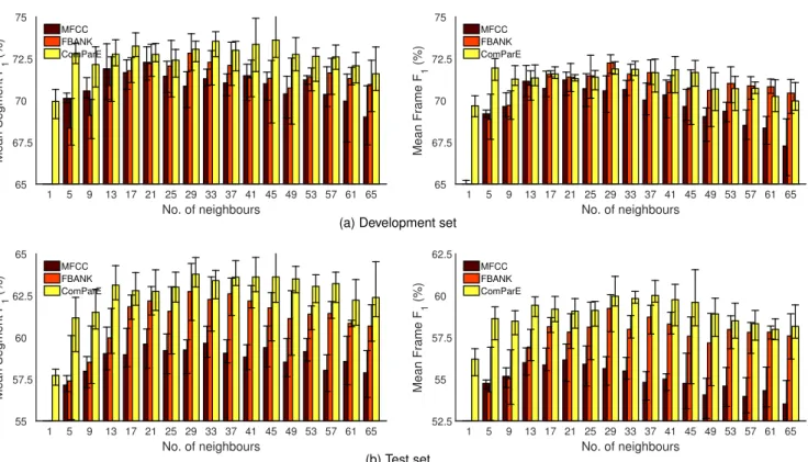
The minimum, maximum, and meanF1scores obtained this way are shown in Fig. 2. It can be seen that concatenat- ing the feature vectors of the neighbouring frames indeed helps classification. We chose the sliding windows with a length of 21, 29 and 33, MFCC, FBANK and ComParE feature sets, respectively. Lowest mean scores were achieved via MFCC, while models trained with FBANK and Com- ParE had roughly the same performance, ComParE pro- ducing slightly higher average values. Taking the minimum and maximum values into consideration as well, we can see that the variation of scores is practically independent of the number of neighbours used or the feature set. In general, however, the segment-level F1 scores tend to vary more than the frame-level scores; in our opinion this is because the key difference between the models trained is reflected in the detection or miss of shorter occurrences. These appear in the frame-level performance values only slightly, but they affect the segment-levelF1 scores more, since at this level an occurrence lasting only a couple of frames is just as important as one being over one second long (which, in our experience, is not unrealistic for a laughter event).

Table 2 contains the precision, recall and F-measure scores measured for the best sliding window sizes (21, 29 and 33, MFCC, FBANK and ComParE feature sets, respectively). The frame-level scores are higher than those reported by Salamin et al. [4], which is probably because we used DNNs for frame-level likelihood estimation, which can be considered as state-of-the-art, while Salamin et al.

used Gaussian Processes. (Note that, despite the fact that

(6)

No. of neighbours

1 5 9 13 17 21 25 29 33 37 41 45 49 53 57 61 65 Mean Segment F 1 (%)

65 67.5 70 72.5 75

MFCC FBANK ComParE

No. of neighbours

1 5 9 13 17 21 25 29 33 37 41 45 49 53 57 61 65 Mean Frame F1 (%)

65 67.5 70 72.5 75

MFCC FBANK ComParE

(a) Development set

No. of neighbours

1 5 9 13 17 21 25 29 33 37 41 45 49 53 57 61 65 Mean Segment F 1 (%)

55 57.5 60 62.5 65

MFCC FBANK ComParE

No. of neighbours

1 5 9 13 17 21 25 29 33 37 41 45 49 53 57 61 65 Mean Frame F1 (%)

52.5 55 57.5 60 62.5

MFCC FBANK ComParE

(b) Test set

Fig. 2. Segment-level and frame-level macro-averagedF₁-scores obtained using standard backpropagation DNN training on the three feature sets applied, as a function of the number of neighbouring frame vectors used during training. The error bars denote minimum and maximumF₁scores.

TABLE 2

Optimal number of neighbouring frames used during training and the corresponding segment- and frame-level precision, recall andF₁scores for both the development and test sets (which will serve as our baseline)

Data No. of Laughter Filler Combined

Evaluation Subset Feature Set frames Prec. Rec. F₁ Prec. Rec. F₁ F₁

Segment-level

MFCC 21 ⁶⁸.8% 64.7% 66.6% 80.1% 75.9% 77.9% 72.3%

Dev. FBANK 29 75.6% 63.4% 69.0% 82.0% 72.0% 76.7% 72.8%

ComParE 33 ⁷⁰.6% 69.3% 69.9% 81.6% 73.2% 77.1% 73.5%

MFCC 21 49.2% 57.8% 53.1% 65.8% 66.0% 65.9% 59.6%

Test FBANK 29 ⁶².9% 57.3% 60.0% 69.2% 62.2% 65.5% 62.7%

ComParE 33 ⁵⁸.0% 62.4% 60.1% 66.3% 67.1% 66.7% 63.4%

Frame-level

Dev.

MFCC 21 ⁶⁷.8% 74.8% 71.1% 67.5% 75.6% 71.3% 71.2%

FBANK 29 ⁶⁹.5% 78.7% 73.8% 66.6% 75.3% 70.7% 72.2%

ComParE 33 ⁷⁰.2% 76.3% 73.0% 70.7% 70.5% 70.6% 71.9%

HMM/GPR [4] — 65.0% 66.0% 65.0% 49.0% 73.0% 59.0% 62.6%

MFCC 21 ⁴³.7% 70.9% 54.0% 52.8% 63.3% 57.6% 56.1%

Test FBANK 29 51.9% 72.3% 60.4% 53.8% 62.4% 57.8% 59.2%

ComParE 33 ⁵⁴.6% 70.4% 61.4% 54.3% 62.6% 58.1% 59.8%

the SSPNet Vocalization corpus is freely available, we found no other study that employed a Hidden Markov Model on it.) Overall, the accuracy scores obtained for laughter events are quite similar to those got for filler events. At the segment level we can see that precision is usually higher than recall, while we got the opposite at the frame level. We can also see that the segment-level scores obtained are higher for filler events than those for laughter, while this is not so when we compute the accuracy metrics at the frame level.

The reason for this is probably that laughter occurrences are usually much longer than filler events. Indeed, in this

corpus, laughter occurrences have an average duration of 942ms, while this is only 502ms for fillers (see Table 1). This difference means that there are three times as many filler event occurrences (segments) as there are laughter events.

However, the number of laughter and filler frames do not differ to such a high extent, and this may lead to a more balanced performance at the frame level.

4.2 Results With Probabilistic Sampling

The averageF1scores achieved by probabilistic sampling on the development set can be seen in Fig. 3; baseline values

(7)

λ

0 0.1 0.2 0.3 0.4 0.5 0.6 0.7 0.8 0.9 1 Mean Segment F 1 (%)

60 65 70 75 80

MFCC FBANK ComParE

λ

0 0.1 0.2 0.3 0.4 0.5 0.6 0.7 0.8 0.9 1 Mean Frame F1 (%)

60 65 70 75 80

MFCC FBANK ComParE

(a) No division by priors

λ

0 0.1 0.2 0.3 0.4 0.5 0.6 0.7 0.8 0.9 1 Mean Segment F 1 (%)

60 65 70 75 80

MFCC FBANK ComParE

λ

0 0.1 0.2 0.3 0.4 0.5 0.6 0.7 0.8 0.9 1 Mean Frame F1 (%)

60 65 70 75 80

MFCC FBANK ComParE

(b) Division by the original priors

λ

0 0.1 0.2 0.3 0.4 0.5 0.6 0.7 0.8 0.9 1 Mean Segment F 1 (%)

60 65 70 75 80

MFCC FBANK ComParE

λ

0 0.1 0.2 0.3 0.4 0.5 0.6 0.7 0.8 0.9 1 Mean Frame F1 (%)

60 65 70 75 80

MFCC FBANK ComParE

(c) Division by the actual priors used during training (i.e. Eq. (1))

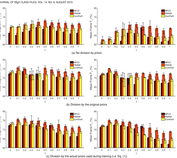
Fig. 3. Mean macro-averagedF₁scores as a function ofλon the development set, at the segment level (left) and frame level (right), when omitting division by the class priors (top), performing division by the original class priors (middle) and by the actual class priors used during training (bottom).

are shown as λ = 0. We can see that models trained on the MFCC feature set performed the worst. Regarding the FBANK and ComParE feature sets, while with the baseline setting (i.e. using full instance sampling) ComParE turned out to be the better one, when we applied probabilistic sampling we got our best scores usually by relying on the FBANK feature vectors. The scores obtained for the latter two feature sets are quite similar, though, so in our opinion any of these two could be used for efficient vocalization localization.

The effect of the three posterior correction strategies tested (i.e. whether we divide the DNN output likelihoods by some class prior values) is also apparent in Fig. 3. When we performed the Viterbi search by relying on the raw likelihoods (see Fig. 3a), the region 0.4 ≤ λ ≤0.6 proved to be best both for the segment-level and for the frame- level scores. As expected,λvalues close to1proved to be better than those near0, perhaps with the exception of the ComParE feature set evaluated at the segment level.

When dividing by the original class priors (see Fig. 3b),

DNNs trained with λ = 0.1 or λ = 0.2 had the highest F1scores both at the segment level and at the frame level.

While for some feature sets there is a drop of accuracy in the region [0.4,0.6], in general lower λ values are better than higher ones. When we transformed the DNN outputs by dividing them by the actual class priors used during training (see Fig. 3c), we can observe a transition between the two previous cases: for λ ≥ 0.7 values, the resulting scores are very close to those obtained via the first strategy;

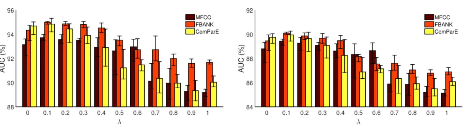
for values λ ≤ 0.2 the scores are close to the second one; while the region in the middle displays a continuous transition between the two. Sinceλvalues above 0.6 usually proved suboptimal even in the case of using the original DNN output likelihoods, this strategy did not work well in this region either. For0.1≤λ≤0.5, however, it performed consistently better than when we divided by the original class priors, leading to the highest scores overall.

Tables 3 and 4 list the precision, recall and F-measure values obtained on the test set with the optimal λ value fine-tuned on the development set, segment and frame-

(8)

TABLE 3

Optimalsegment-levelF₁and the corresponding precision and recall scores on the test set for the two sampling techniques tested

Feature Sampling Div. Laughter Filler Combined Opt.

set method priors Prec. Rec. F₁ Prec. Rec. F₁ F₁ p λ

MFCC

Probabilistic

no 53.1% 66.0% 58.6% 62.0% 68.5% 65.1% 62.0% = 0.03 0.6 yes ⁵¹.7% 64.1% 57.0% 64.3% 67.3% 65.7% 61.5% = 0.03 0.2

actual 55.7% 67.4% 61.0% 65.4% 66.1% 65.6% 63.5% <0.01 0.3

Downsampling no ⁵¹.7% 63.6% 57.0% 62.1% 67.7% 64.7% 60.9% = 0.03 — Full (baseline) yes ⁴⁹.2% 57.8% 53.1% 65.8% ⁶⁶.0% 65.9% ⁵⁹.6% — —

FBANK

Probabilistic

no 64.5% ⁶⁵.6% 65.0% ⁶⁷.3% 65.5% 66.3% 65.7% <0.01 0.5 yes 57.8% 67.1% 61.9% 67.0% 67.3% 67.0% 64.6% = 0.03 0.1 actual 64.4% ⁶⁴.1% 64.2% 68.9% 63.8% 66.2% 65.3% = 0.02 0.2

Downsampling no 51.7% 63.9% 57.2% 64.6% 67.4% 65.9% 61.7% — —

Full (baseline) yes ⁶².9% 57.3% 60.0% 69.2% ⁶².2% 65.5% 62.7% — —

ComParE

Probabilistic

no 59.7% ⁶⁵.7% 62.3% 69.1% ⁶⁰.5% 64.4% 63.7% = 0.84 0.3 yes ⁵⁴.9% 70.0% ⁶¹.3% 67.3% 65.2% 66.2% 64.1% = 0.69 0.1 actual ⁵⁸.1% 69.9% 63.1% ⁶⁸.2% 65.2% 66.6% 65.2% <0.01 0.2 Downsampling no ⁵⁴.2% 66.9% 59.8% 67.1% 66.1% 66.5% 63.4% — —

Full (baseline) yes 58.0% 62.4% 60.1% 66.3% 67.1% 66.7% 63.4% — —

TABLE 4

Optimalframe-levelF₁and the corresponding precision and recall scores on the test set for the two sampling techniques tested

Feature Sampling Div. Laughter Filler Combined Opt.

set method priors Prec. Rec. F₁ Prec. Rec. F₁ F₁ p λ

MFCC

Probabilistic

no 62.5% ⁵⁶.2% 59.0% 58.3% ⁵⁸.1% 58.1% 58.6% <0.01 0.6 yes ⁵³.6% 67.2% 59.6% 56.8% 60.9% 58.8% ⁵⁹.3% <0.01 0.1 actual ⁶⁰.5% 62.2% 61.3% ⁵⁶.5% 61.5% 58.8% 60.1% <0.01 0.2

Downsampling no 46.8% 72.0% 56.7% 48.1% 64.2% 55.0% 55.9% — —

Full (baseline) yes ⁴³.7% 70.9% 54.0% 52.8% 63.3% 57.6% 56.1% — —

FBANK

Probabilistic

no 71.7% ⁵⁵.0% 62.3% 59.6% 58.2% 58.9% 60.8% = 0.03 0.5 yes ⁵⁸.0% 71.6% 64.0% 58.9% 61.8% 60.3% 62.3% <0.01 0.1 actual ⁶³.2% 66.4% 64.7% 60.1% ⁵⁹.6% 59.8% 62.3% <0.01 0.2

Downsampling no ⁴⁸.6% 73.5% ⁵⁸.5% 47.9% 64.9% ⁵⁵.1% 56.8% — —

Full (baseline) yes ⁵¹.9% 72.3% 60.4% 53.8% 62.4% 57.8% 59.2% — —

ComParE

Probabilistic

no 66.9% 54.9% 60.2% 62.5% 53.7% 57.7% 59.0% — 0.3

yes ⁵⁴.5% 74.1% 62.4% 58.5% 61.0% 59.7% 61.5% = 0.02 0.1

actual 60.1% 68.0% 63.4% 60.2% 60.4% 60.2% 62.0% <0.01 0.1

Downsampling no ⁴⁹.2% 75.4% ⁵⁹.5% 52.5% 64.8% ⁵⁸.0% 58.9% — —

Full (baseline) yes 54.6% 70.4% 61.4% 54.3% 62.6% 58.1% 59.8% — —

level scores, respectively. (The best scores are shown in bold.) We also indicated the statistical significance (p) of the improvements (if any) by using a Mann-WhitneyUtest [50].

We can see that on the test set, depending on the feature set, the segment-level scores increased by 2.6–3.9% absolute, while the frame-level scores rose by 2.2–4.0% compared to the corresponding baseline values. These gains mean a relative error reduction score of between 5–10% and 5–9% at the segment level and frame level, respectively; the highest scores achieved by utilizing probabilistic sampling (using the FBANK feature set and dividing the output likelihoods by the actual class priors used during training) brought a 7% and a8%relative error reduction over the baseline. It is interesting to note that most of the improvement came from detecting the laughter events, while the metric values associated with the filler events improved only slightly

(or sometimes not at all). Recall (see Table 1) that only 3.4% of the training frames were laughter events, while fillers accounted for 50% more than that (4.9%), hence it is quite understandable that probabilistic sampling helped the detection of the former event types more.

For comparison, we also tested the simple sampling approach of downsampling. We realized downsampling by randomly discarding samples from the “garbage” class to make its frequency match that of filler frames. We got the best results by avoiding the division of the obtained posterior values by the class priors (see tables 3 and 4). Still, the performance of downsampling practically matched that of the baseline, i.e. full database sampling at the segment level, while at the level of frames this strategy even led to somewhat worse F1 values. In our opinion this indicates the downsampling approach is just too simple to improve

(9)

No. of neighbours

1 5 9 13 17 21 25 29 33 37 41 45 49 53 57 61 65

AUC (%)

88 90 92 94 96

MFCC FBANK ComParE

No. of neighbours

1 5 9 13 17 21 25 29 33 37 41 45 49 53 57 61 65

AUC (%)

84 86 88 90 92

MFCC FBANK ComParE

Fig. 4. Averaged AUC values obtained using standard backpropagation DNN training as a function of the number of neighbouring frame vectors used during training, on the development set (left) and on the test set (right).

TABLE 5

The obtained AUC scores using standard backpropagation DNN training for both the development and test sets, and some notable results published in the literature on this dataset

No. of Development Test

Approach Feature Set frames Lau. Fil. Avg. Lau. Fil. Avg.

MFCC 21 ⁹¹.6% 94.8% 93.2% 89.7% 87.6% 88.7%

DNN (optimalF₁) FBANK 29 ⁹³.3% 95.4% 94.4% 90.6% 88.1% 89.3%

ComParE 33 ⁹².7% 95.5% 94.1% 91.0% 87.7% 89.4%

MFCC 53 ⁹².6% 95.3% 94.0% 90.2% 86.3% 88.3%

DNN (optimal AUC) FBANK 53 94.2% 96.1% 95.2% 91.0% 87.7% 89.4%

ComParE 53 ⁹³.3% 96.0% 94.6% 91.4% 88.0% 89.7%

ComParE baseline (Schuller et al. [10]) ⁸⁶.2% 89.0% 87.6% 82.9% 83.6% 83.3%

DNN downsampling (Gupta et al. [5]) ⁹⁰.1% 90.1% 90.1% — — —

DNN + smoothing + masking (Gupta et al. [5]) ⁹⁵.1% 94.7% 94.9% 93.3% 89.7% 91.5%

DNN + DNN (Brueckner and Schuller [34]) ⁹⁸.1% 96.5% 97.3% 94.9% 89.9% 92.4%

BLSTM (Brueckner and Schuller [36]) — — 97.0% — — 93.0%

DNN + GA smoothing (Gosztolya [51]) ⁹⁷.5% 96.7% 97.1% 96.0% 90.1% 93.1%

DNN + BLSTM smoothing (Brueckner and Schuller [36]) — — 97.2% — — 94.0%

performance in this task, probably because it reduced the variance of the “garbage” class to a great extent.

Overall, the application of probabilistic sampling gave a significant improvement both at the segment and at the frame levels. (The improvements were found to be significant at the level p < 0.01 in all but one case, the only exception being the segment-levelF1values using the FBANK feature set withp= 0.0159.) Instead of the extreme values ofλ = 0 andλ = 1, corresponding to the original and the uniform class distributions, optimal performance was always achieved with intermediateλvalues. A possible reason is that, since we do not generate further examples of the rarer classes for training, we have to use our samples more frequently. Because of this, we actually use examples belonging to the more frequent classes less frequently (actually, not all samples are used for each iteration), which decreases the variance of such classes. By changing the λ parameter value, we can establish a trade-off between the two extremes, which seems to work quite well in practice.

5 RESULTS USING AUC

Although we primarily measure the accuracy of DNN models trained by calculating segment and frame-level precision, recall andF1values after using a Hidden Markov Model, as

we find this approach more meaningful, next we will also present the frame-level AUC scores obtained for reference.

5.1 Baseline Scores

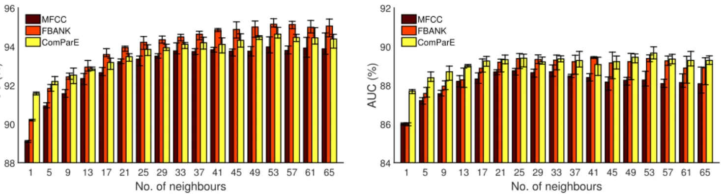
Fig. 4 shows the AUC values obtained on the development and on the test set as a function of the number of neighbouring frame vectors used for all three feature sets tested. We can see that on the development set, the AUC values show an increasing trend even when we use over 50 neighbouring frames, while on the test set the scores stop increasing after about 20 frames, or in the case of the MFCC features they even start to decrease. The reason for this cannot be any form of overfitting, since no meta-parameter setting has yet been applied on the development set; in our opinion, this behaviour suggests there is a mismatch between the development and test sets of this particular database.

Table 5 lists the AUC scores of the DNN models trained via standard backpropagation and full database sampling.

We can see that if we chose the number of neighbouring frame vectors based on the optimalF1 value on the development set (i.e. following Fig. 2 and Table 2), we ended up using fewer neighbouring frame vectors (between 21 and 33) than when we chose the size of neighbourhood based on the optimal AUC value on the development set,