T for Buckling of High Strength Steel Welded Box Section Columns Comparison of Safety Factor Evaluation Methods

(1)



Abstract—In the research praxis of civil engineering, the statistical evaluation of experimental and numerical investigations is an essential task in order to compare the resistance of a specific structural problem with the proposed resistance of the standards. However, in the standards and in the international literature there are several different safety factor evaluation methods that can be used to check the necessary safety level (e.g.: 5% quantile level, 2.3% quantile level, 1‰

quantile level, γM partial safety factor, γM* partial safety factor, β reliability index). Moreover, in the international literature, different calculation methods could be found even for the same safety factor as well. In the present study, the flexural buckling resistance of high strength steel (HSS) welded closed sections are analyzed. The authors investigated the flexural buckling resistances of the analyzed columns by laboratory experiments. In the present study, the safety levels of the obtained experimental resistances are calculated based on several safety approaches and compared with the EN 1990. The results of the different safety approaches are compared and evaluated. It is concluded that for statistical evaluation of experimental results subdividing the evaluated groups is advantageous. Based on the evaluation tendencies are identified and the differences between the statistical evaluation methods are explained. Moreover, the results show that that higher steel grades provide higher safety level than lower steel grades.

Keywords—Flexural buckling, high strength steel, partial safety factor, statistical evaluation.

I. INTRODUCTION

HE statistical evaluation is an essential task in design of civil engineering structures. In Europe the necessary safety criteria is defined in the EN 1990 [1] for all materials (steel, concrete, timber, glass, etc.). The theoretical base of the defined safety is based on the reliability of load and resistance together applying the β reliability index using full probabilistic design method. It means that the safety level of a design resistance model depends on the actual loading situations, therefore, the safety level depends on the application area of the structure.

However, the general aim by the development of a design method to determine a specific resistance that should be used on the same way for all structures independently from the application area, and the method should provide a general safety level for all cases. This need is in contrast with the application of the full probabilistic design method. This is already recognized by the creators of the European standards, therefore in EN 1990 [1] the load and resistance sides are separated from each other creating a semi-probabilistic design B. Somodi and B. Kövesdi are with the Department of Structural Engineering, Faculty of Civil Engineering, Budapest University of Technology

method. This results in that a design resistance model could be evaluated without taking into consideration the application area and the loading situation. However, in the literature several semi-probabilistic methods could be found or used in the past to define safety criterion for a design resistance model, and these methods provide different safety levels.

In the present paper semi-probabilistic reliability assessment methodologies are collected and used to define the safety level of the flexural buckling curves of the EN 1993-1-1 [2] for axially compressed welded square box section columns based on experimental results. The experimental test set contained columns made of conventional mild steels from S235 up to S460 material grades (NSS – normal strength steel) and columns made of high strength steels (HSS) from S500 up to S960 steel grades.

II. RELIABILITY ASSESSMENT METHODS A. Full probabilistic design method – probability failure and β reliability index

According to EN 1990 [1] the reliability of a structural element or a whole structure should be ensured by controlling the probability of failure (Pf) using the reliability index (β).

Applying the defined methodology, the structure or structural element should safely resist the loading actions and should fulfill all the requirements defined by the standard. In order to avoid the failure of the structure the resistance values (R) should be always equal or higher than the related effect of actions (E), therefore the probability of the failure is defined as the probability of the case when R < E, see (1).

) P 0)

( (g

Pf P RE   (1)

The g reliability function (or limit state function) is defined as the difference of the resistance and the effect of actions (g = R – E). If it gives negative value, then structural failure occurs.

The EN 1990 assumes that the reliability function has a Gaussian distribution, which mean value is μg, and its standard deviation is σg. Using these assumptions the reliability index is defined by (2).

g g



 (2)

So the β reliability index basically defines that the distance between the mean value and the failure limit is how much time of the standard deviation. If β is higher, then the failure is

and Economics, Budapest, Hungary (e-mail: somodi.balazs@epito.bme.hu, kovesdi.balazs@epito.bme.hu).

Balázs Somodi, Balázs Kövesdi

Comparison of Safety Factor Evaluation Methods for Buckling of High Strength Steel Welded Box

Section Columns

T

(2)

further of the mean value, thus the safety level is higher. The connection between the reliability index and the failure probability is demonstrated in Table I. Using the Φ cumulative distribution function of the standardized normal distribution the probabilistic of the failure can be expressed by (3).

( )

Pf    (3)

TABLEI

RELIABILITY INDEX AND FAILURE PROBABILITY

β 1.282 2.326 3.090 3.719 4.265 4.753 5.199 Pf 1E-01 1E-02 1E-03 1E-04 1E-05 1E-06 1E-07 The EN 1990 [1] specifies the minimum values of β in dependence of the reference period and of the reliability class.

In case of the mainly used Reliability Class 2 (RC2), the yearly accepted and recommended failure probability equals to 10^-6, which corresponds to β = 4.75 according to Table I.

Considering the usually applied reference period as 50 years the yearly Pf = 10^-6 results in β = 3.8.

B. Semi-probabilistic design methods – separation of action and resistance side

The previously introduced full probabilistic method is a whole and appropriate reliability principle. However, it is not practical for codification purposes, because the design resistance models should provide appropriate regulations for all types of structures independently from application and location.

Therefore, the loading side and the resistance side of the reliability assessment should be separated from each other.

The EN 1990 [1] introduces the semi-probabilistic design method by separating the total β reliability index into two parts.

The αRβ should be used only for the resistance part and αEβ should be used for the action side. The factors are defined as αR

= 0.8 and αE = 0.7, therefore the total reliability index remains almost the same, see (4).

2 2 1.063

R E

     (4)

This method allows to evaluate the resistance side independently from the actions and to obtain appropriate γM

partial factors only by analyzing the resistances. Using this methodology, the failure is defined if the actual resistance is lower than its design value (R < Rd), so the probability of failure caused by lack of resistance is defined by (5) instead of (1) and (3).

)

( _d ( )

f R

P PRR    (5)

It means that the design value of a certain resistance component should be defined so as the required reliability index on the resistance side equals to αRβ, which is 0.8 × 3.8 = 3.04 assuming reliability class RC2 and a reference period of 50 years. In this case (RC2, and 50 years) the design resistance value should be defined as the lower 0.118% quantile of the resistance function, since Φ(3.04) = 1/845 = 1.18‰, which means that no more than one out of 845 elements may have lower resistance than the design resistance.

III. STATISTICAL DETERMINATION OF RESISTANCE MODEL All of the applied semi-probabilistic design methods that are

used in this paper and introduced in Section IV are using the basics of the EN 1990: Annex D [1]. These are summarized in this Section. The actual resistance value of a certain structural element is defined by (6).

rbrt (6)

where:

b is the mean value correction factor, rt is the theoretical resistance, δ is the error term.

The rt theoretical resistance can be calculated from the resistance function by (7), which is a function of the Xi basic variables that affect the resistance. The mean value correction factor (b) can be calculated by the comparison of the measured resistances (re) and the theoretical values calculated by the resistance function using the actual measured properties (rt), see (8).

( )

t rt i

rg X (7)

, ,

2 , e i t i

t i

r r

b r









⁽⁸⁾

Using (6), the error term (δi) for each experimental test should be calculated by (9).

, , e i i

t i

r

 b r



(9) From the individual error terms, the coefficient of variation (CoV) of the error (Vδ) can be determined as follows, see (10).

exp( 2) 1

V_ s_  (10)

where:

2 2

1

1 ( )

1

n i i

s^ n 

   





⁽¹¹⁾

1

1 ⁿ

i

ni

 



 ⁽¹²⁾

ln( )

i i

  (13)

In the equations above n is the number of the experimental tests.

The EN 1990: Annex D [1] specifies how to calculate the characteristic and design values of the resistance from experimental tests knowing the Vδ CoV of the error term. If a large number of tests is available, the characteristic resistance (rk) may be calculated by (14) and the design resistance (rd) can be obtained by (15).

( ) exp( 0.5 2)

k rt m

r  b g X k Q  Q (14)

2

( ) exp( , 0.5 )

d rt m d

r  b g X k _Q Q (15)

where:

 grt(Xm) is the theoretical resistance calculated by the resistance function using the mean values of the basic variables,

 kd,∞ = 3.04 in agreement with the value that is defined at the end of Section II,

 k∞ = 1.64, the characteristic value is defined as the lower 5% of the experimental resistances, since Φ(1.64) = 1/19.8

= 5.05%, which means that no more than one out of 20 elements may have lower resistance than the characteristic resistance,

(3)

 _ln( ² ₁₎

Q Vr  (16)

Vr is the total CoV that includes the CoV of the error term (Vδ) and the CoV of the basic variables (VXi) that can be calculated by (17) and (18) if the affecting CoV values are small.

2 2 2

r rt

V V_ V (17)

2 2

rt Xi

i

V 



V ⁽¹⁸⁾

The VXi CoV of the basic variables usually need to be determined on the basis of some prior knowledge. Those can be calculated from the test data only if the test population fully represents the variation of the reality. In the current paper the CoV of the basic variables are taken into account based on the suggestion of JCSS [3], see (19), (20), (21).

fy 0.07

V  - yield strength (19)

t 0.05

V  - plate thickness (20)

0.005

Vb - width of the cross-section (21)

Equations (14) and (15) are applicable if a large number of tests results are available. The EN 1990: Annex D [1] specifies the large number as n ≥ 100, but the alternative calculation method for smaller test number provides the same results if n >

30 considering that the Table D1 of EN 1990: Annex D [1]

gives the k∞ for kn if n > 30. Practically the introduced calculation method for the characteristic and design resistances is valid if there are more than 30 test results are available.

If the introduced calculation method results in too high Vδ, then the scatter may be reduced by dividing the total test population into appropriate sub-sets. When calculating the statistical parameters of the sub-sets, the number of the test results (n) can be considered equal to the total number of tests in the original series. The statistical evaluation of the entire test set without subdividing them into sub-sets results in a conservative result, as shown by da Silva et al. [4]. Therefore, the calculated safety factors are calculated for different steel grade groups. Moreover, the available test results for each steel grade groups are grouped into subgroups based on the global slenderness ratio. For all the subgroups the same evaluation process is executed and the final partial safety factor for each steel grade group is determined by averaging the safety factors of the subgroups. The evaluation without subgrouping is also made for comparison purpose.

IV. APPLIED SEMI-PROBABILISTIC DESIGN METHODS A. Method A - γM*

The first method that is used in present paper is identified as Method A. The method is used or presented by Taras and da Silva [5], da Silva et al. [6], da Silva et al. [4], Heinisuo [7], Taras and Huemer [8] and Schillo [9]. This method ensures that the design value of the examined population is determined using the proposed buckling curve and the predefined partial safety factor. Based on this method, the required partial safety factor applicable for designs (γM*) can be calculated based on the nominal resistance and the design resistance by (22).

nom M

d

r

 ^ r (22)

where rd is defined by (15) and rnom can be calculated in function of the nominal values of the basic parameters (Xnom) using the resistance function by (23).

( )

nom rt nom

r g X (23)

The partial safety factor is determined differently for all experimental tests. The average partial safety factor should be determined for all sub-set separately, and the final safety factor should be calculated as the mean value of the averaged γM*

partial safety factors of the individual sub-sets.

The relevant safety factor for column buckling in EN1993-1- 1 [2] is equal to 1.0 for buildings and 1.1 for bridges. In [10]

γM1*=1.1 is proposed, but the code still uses γM1*=1.0 for buildings. If the calculated γM1* is lower than 1.0 based on the statistical evaluation of test results, the examined resistance model meets the standard safety criteria of the current EN 1990 [1]. If γM1* is between 1.0 and 1.1, then the examined resistance model does not meet the safety criteria, but still reaches the same safety level that is provided by the current EN1993-1-1 [2]. If the calculated γM1* is higher than 1.1, the necessary safety level of the examined resistance model cannot be justified.

B. Method B - γM*

The second method that is used in present paper is identified as Method B. The method is used by Johansson et al. [11], Johansson et al. [12], by European background documents [10]

and by Somodi and Kövesdi [13], [14], [15]. This method is also based on the γM* partial safety factor, therefore, the basic statements are also true that is introduced for Method A.

However, Method B gives a different calculation method for the value of γM*. The required partial safety factor applicable for designs (γM*) can be calculated based on the theoretical partial safety factor (γM) and a modification factor (Δk) by (24). The modification factor considers that the characteristic value for the input parameters is used as the nominal value instead of the lower 5% quantile value in most cases.

M k M

 ^   (24)

where:

exp(1.4 )

k M

d

r Q

 r  (25)

2

2 2

exp( 2 0.5 ) 0.867

exp( k 0.5 ) exp( 1.64 0.5 )

fy fy

Q Q

k b _Q Q b Q Q

 

  

      (26)

where Q is defined by (16) and Qfy is considered to be equal to 0.07 based on JCSS [3].

Using this method only one γM* is calculated for each sub-set (no different values for each experimental test), and the final safety factor should be calculated as the mean value of the γM*

partial safety factors of the individual sub-sets. The target values of the partial safety factor are the same as it is introduced in the previous section.

C. Method C – k2.3%

The third method that is used in the present paper is identified as Method C. The method is used by the evaluation of the current column buckling curves in the EN1993-1-1 [2] and used

(4)

by Somodi and Kövesdi [13], [14], [15].

According to this method the lower 2.3% quantiles (mean value minus two times standard deviation) of the experimental results are determined and proposed as the relevant column buckling curve. In frame of this method a k2.3% safety factor is determined for the examined subgroups by (27).

2.3% (1 _n )

k   b k V_ (27)

where kn is equal to 2.0, the values of b and Vδ are defined by (8) and (10). If the criterion of k2.3% ≥ 1.0 is met, the necessary safety is ensured and the column buckling curve can be used in the design.

V. PREVIOUS EXPERIMENTAL PROGRAM

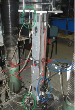
A total of 49 global column buckling tests on welded box section columns were carried out at the Budapest University of Technology and Economics, Department of Structural Engineering between 2015-16 [13]. All the test specimens fulfilled the requirements of cross section class 3, therefore no local buckling occurred during the tests. A total of 18 different cross section geometries made from welded square box sections were investigated using 7 different steel grades (S235, S355, S420, S460, S500, S700 and S960). The experimental research program is unique in the field of the buckling behaviour of HSS columns, because NSS and HSS columns were tested using the same loading and supporting conditions, the same testing rigs and manufacturing process. The same boundary conditions ensured the comparability of the buckling resistances and to evaluate their differences. The specimens are tested using hinged support conditions. The test set-up is shown in Fig. 1.

Fig. 1 Flexural buckling test layout and test specimen For each specimen the followings are measured to be able to evaluate the buckling test results and to determine the appropriate column buckling curve:

 residual stresses for each cross section geometries for all analyzed steel grades, see [16] and [17],

 global geometrical imperfections (out-of-plane straightness) for each specimen,

 loading eccentricities for each specimen,

 material properties for each analyzed steel grades and plate thicknesses,

 load-displacement diagrams regarding longitudinal and lateral displacements,

 stress distribution within the cross-section to check the local buckling phenomenon.

The observed failure modes were always pure flexural buckling without any interaction with local buckling failure modes. The exact shape of all the test specimens are measured prior the buckling tests. The shape and magnitude of the imperfection are measured on each corner of all test specimens.

The measurements showed that the out-of-straightness imperfections are significantly smaller than the manufacturing tolerance given by the Eurocode (L/750), and its values varied between L/10000 - L/1000. No clear tendencies in the imperfection magnitudes could be observed depending on the steel grade and depending on the global slenderness. The average measured out-of-straightness imperfection magnitude was about L/3000. In present paper 39 of the 49 tested columns are used for the statistical evaluation, the measured flexural buckling resistances of these specimens are plotted in Fig. 2, where χtest is calculated based on the measured geometries and material properties for each test specimen. More details about the experimental research program, about the geometry of the test specimens and the measured results are published in [13] in a detailed manner.

Fig. 2 Buckling reduction factors (χtest) based on actual values.

VI. SAFETY ANALYSIS

As a comprehensive safety analysis, the safety levels are calculated based on all of the three semi-probabilistic design methods that are introduced in Section IV for all investigated cases. The experimental results are grouped into five different groups based on the material grades and the reliability assessment is done for all of these groups separately. The following steel grade groups are specified:

(5)

 All steel grades – 39 specimens

 HSS grades (S500, S700, S960) – 7 specimens

 NSS grades (S235, S355, S420, S460) – 32 specimens

 NSS grades with higher fy (S420, S460) – 13 specimens

 Conventional steel grades (S235, S355) – 19 specimens The steel grade groups are divided into subsets based on the slenderness ratio and the evaluation is made considering these sub-sets as introduced in Section III. The following sub-sets are applied:

 Sub-set 1 – 0.5 < λ ≤ 0.65

 Sub-set 2 – 0.65 < λ ≤ 0.8

 Sub-set 3 – 0.8 < λ ≤ 1.0

 Sub-set 4 – 1.0 < λ

For the groups of the HSS grades the sub-sets 1 & 2 and the sub-sets 3 & 4 are merged because of the smaller number of test specimens.

To obtain the final safety factor of a steel grade group, the calculated safety factors of the sub-sets should be averaged. The averaging is done in two ways:

 simple arithmetic mean,

 weighted arithmetic mean by the slenderness range.

TABLEII

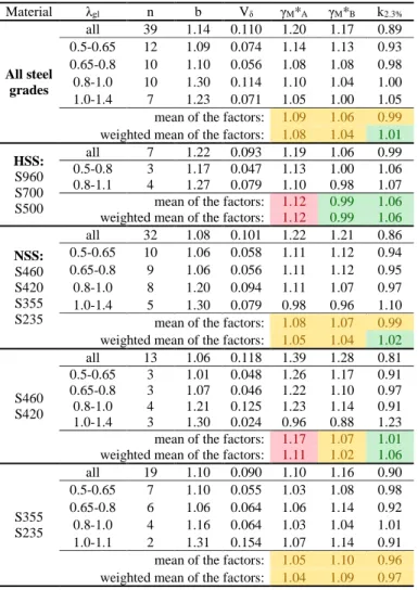
STATISTICAL PARAMETERS AND SAFETY FACTORS FOR CURVE C Material λgl n b Vδ γM*A γM*B k2.3%

All steel grades

all 39 1.23 0.120 1.15 1.11 0.94 0.5-0.65 12 1.16 0.072 1.08 1.05 1.00 0.65-0.8 10 1.20 0.058 1.00 0.99 1.06 0.8-1.0 10 1.43 0.114 1.00 0.95 1.10 1.0-1.4 7 1.36 0.072 0.95 0.90 1.16 mean of the factors: 1.01 0.97 1.08 weighted mean of the factors: 0.99 0.95 1.10 HSS:

S960 S700 S500

all 7 1.33 0.103 1.12 0.99 1.05 0.5-0.8 3 1.26 0.030 1.03 0.91 1.19 0.8-1.1 4 1.40 0.077 1.00 0.88 1.19 mean of the factors: 1.01 0.90 1.19 weighted mean of the factors: 1.01 0.90 1.19

NSS:

S460 S420 S355 S235

all 32 1.16 0.111 1.17 1.15 0.90 0.5-0.65 10 1.13 0.055 1.05 1.05 1.01 0.65-0.8 9 1.16 0.057 1.03 1.03 1.02 0.8-1.0 8 1.32 0.094 1.01 0.97 1.07 1.0-1.4 5 1.43 0.080 0.89 0.87 1.21 mean of the factors: 1.00 0.98 1.08 weighted mean of the factors: 0.97 0.95 1.11

S460 S420

S355 S235

all 19 1.17 0.099 1.07 1.11 0.94 0.5-0.65 7 1.17 0.054 0.98 1.02 1.04 0.65-0.8 6 1.15 0.066 0.99 1.05 1.00 0.8-1.0 4 1.28 0.064 0.95 0.95 1.11 1.0-1.1 2 1.45 0.154 0.97 1.04 1.00 mean of the factors: 0.97 1.01 1.04 weighted mean of the factors: 0.97 1.00 1.05 The flexural buckling resistance of the examined welded box section columns should be calculated using buckling curve c of

the EN 1993-1-1 [2] based on the current European standard.

Therefore, the safety factors are calculated for the resistance model using buckling curve c, these are shown in Table II.

The final safety factors are highlighted with colorful background. Green background means that the safety criteria are met. For the partial safety factor, the background is yellow, if it is between 1.00 and 1.10. It means that the test population reaches the safety level of the current standard. Red background means that γM*>1.1. For the k2.3% the background is yellow, if the safety factor is between 1.00 and 0.95, red background means that k2.3%<0.95.

TABLEIII

STATISTICAL PARAMETERS AND SAFETY FACTORS FOR CURVE B Material λgl n b Vδ γM*A γM*B k2.3%

S960 S700 S500

NSS:

S460 S420 S355 S235

S460 S420

S355 S235

all 19 1.10 0.090 1.10 1.16 0.90 0.5-0.65 7 1.10 0.055 1.03 1.08 0.98 0.65-0.8 6 1.06 0.064 1.06 1.14 0.92 0.8-1.0 4 1.16 0.064 1.03 1.04 1.01 1.0-1.1 2 1.31 0.154 1.07 1.14 0.91 mean of the factors: 1.05 1.10 0.96 weighted mean of the factors: 1.04 1.09 0.97 Table II shows that based on almost all grouping and all statistical methods the necessary safety level is met using the buckling curve c. However, the results show that based on Method B and C the cases with HSS grades provides too conservative results, k2.3% ≈ 1.2, which means that the lower 2.3% quantile of the experimental results provide 20% higher resistance than given by the resistance model. Therefore, for these cases higher buckling curves could provide higher flexural buckling resistance with sufficient safety level. In order to examine this presumption, the safety factors also generated based on resistance models using buckling curve b and a of the EN 1993-1-1 [2], these results are shown in Table III and in Table IV. The results show that the necessary safety level

(6)

cannot be ensured using buckling curve a, but the resistance based on the buckling curve b shows sufficient safety level for the following cases:

 HSS grades based on Method B and C,

 S420 – S460 grades based on Method C, based on Method B the safety level still reaches the actual safety level of the EN 1993-1-1 [2].

However, the necessary safety cannot be ensured for these cases using Method A. A tendency can be observed that higher steel grades could be considered using higher buckling curves.

This fact is clearly visible based on Method B and C, however, Method A suggests opposite behavior.

TABLEIV

STATISTICAL PARAMETERS AND SAFETY FACTORS FOR CURVE A Material λgl n b Vδ γM*A γM*B k2.3%

S960 S700 S500

NSS:

S460 S420 S355 S235

S460 S420

S355 S235

VII. CONCLUSIONS A. Effect of subdividing groups

The calculated safety factors show that the statistical evaluation without subdividing groups results in always lower safety level than using sub-sets. By comparing the safety factors provided by Method A and B, using buckling curve c, with and without sub-dividing the steel grade groups (see Fig. 3), it can be observed that omitting the sub-dividing results in always higher partial safety factors, therefore using it to verify a design method results in too conservative design.

Fig. 3 Effect of sub-dividing groups B. Difference between Method A and Method B

Method A and Method B both relies on the γM* partial safety factors, but their calculation method is different. The current results show (see Fig. 4) that Method A provides higher factors for S420 – S960 material grades than Method B, therefore it provides more conservative design. However, in case of S235 – S355 material grades this tendency reverses, and Method A provides lower factors than Method B. In order to explain this behavior, the calculation procedure of the methods has to be analyzed. The Method A derives the partial safety factor from the nominal resistances of the test specimens, therefore, its partial safety factor highly depends on the ratio between the nominal and the actual yield strength of the test specimens.

However, Method B calculates the partial safety factor based on the presumption, that in the reality the manufacturers produce the steel material according to the proposed scattering (νfy = 0.07) of the JCSS [3].

Fig. 4 Comparison of Method A and Method B

Based on the currently analyzed test set the ratios (kfy) between the nominal and actual yield strength are calculated by (28). The kfy is 1.05 for the HSS specimens, 1.09 for the S420 – S460 specimens, but 1.27 for the S235 – S355 specimens. The big difference between the conventional steel grades and the higher steel grades explain the behavior between the Method A and Method B, because there is inverse relation between kfy and

0.80 0.90 1.00 1.10 1.20 1.30 1.40

All HSS NSS S420-S460 S235-S355

Safety factor

A method - all slenderness A method - sub-divided B method - all slenderness B method - sub-divided

0.80 0.85 0.90 0.95 1.00 1.05 1.10 1.15 1.20

HSS S420-S460 S235-S355

Safety factor

Method A - curve b Method A - curve c Method B - curve b Method B - curve c

(7)

the γM* based on the Method A, however, kfy does not affect the γM* based on the Method B.

, ,

1 , ,

n y act i

i y nom i

fy

f k f

n







(28) C. Connection between Method C and methods using γM*

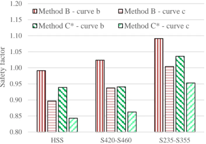
The relation between the k2.3% and the γM* is inverse, because the examined resistance model met the safety criteria if k2.3% ≥ 1.0 and/or if γM* ≤ 1.0. Therefore 1/k2.3% is more easily comparable with γM* than k2.3%. In Fig. 5 the γM* values provided by the Method B and the 1/k2.3% values (labelled as Method C*) are compared using buckling curve b and buckling curve c. The figure shows that Method B and Method C has a good relation with each other. The difference between them is that Method C provides slightly higher safety level, therefore, verifying a design method using Method C always provides slightly less conservative design method than using Method B. Based on the results it can be concluded that the case of k2.3% = 1.0 (so if the safety criteria are just met based on Method C) provides approximately equivalent safety level as it is given by Method B if γM* ≈ 1.05. The connection between Method C and Method A is much more complex, but it can be explained by the facts that is already described is the subsection B.

Fig. 5 Comparison of Method B and Method C

D. Effect of the material grade

The tendency over the different steel grades in Fig 5. clearly shows that higher steel grades provide higher safety level. This observation supports the previous results of Somodi and Kövesdi [13], [14], [15].

VIII. SUMMARY AND NEW FINDINGS

In the present paper three different semi-probabilistic reliability assessment methods (labelled as Method A, B and C) are compared and used to define the safety level of the flexural buckling curve c, b and a of the EN 1993-1-1 [2] for axially compressed welded square box section columns based on previous test results. The experimental program contained columns made of conventional mild steels from S235 up to S460 material grades (NSS – normal strength steel) and

columns made of high strength steels (HSS) from S500 up to S960 material grades. Based on the safety analysis the following conclusions are drawn:

 By the execution of a statistical analysis the test set is suggested to divide into sub-sets, because omitting the subdividing results in much higher partial safety factors.

 Method A highly depends on the ratios between the nominal and actual yield strength of the specimens. If the actual yield strength is much higher than the nominal value, then the method provides high safety level and vice versa, independently from the ratios between the experimental and the calculated resistance based on the actual parameters.

 However, the safety level of Method B depends on the ratios between the experimental resistance and the calculated resistance based on the actual parameters, but it is not affected by the ratios between the nominal and actual yield strength of the test specimens. Therefore, the authors suggest to use Method B instead of Method A.

 The Method C behaves similarly as Method B, but provides slightly higher safety level and verifying a design method using Method C provides slightly less conservative design method than using Method B.

 The case k2.3% = 1.0 by Method C provides approximately equivalent safety level as the case of γM* ≈ 1.05 by Method B.

 The results show that higher steel grades provide higher safety level than lower steel grades using the same resistance model.

ACKNOWLEDGMENT

The executed research program was supported by the ÚNKP-17-3-III and the ÚNKP-17-4-III New National Excellence Program of the Ministry of Human Capacities and by the Campus Mundi Scholarship of the Tempus Public Foundation; the financial support is gratefully acknowledged.

REFERENCES

[1] EN 1990, Eurocode: Basis of structural design, CEN, 2011.

[2] EN 1993-1-1, Eurocode 3: Design of steel structures - Part 1.1: General rules and rules for buildings, CEN, 2011.

[3] Joint Committee of Structural Safety (JCSS), Probabilistic model code, Internet Publication, 2002.

[4] L. S. da Silva, T. Tankova, J. Canha, L. Marques, C. Rebelo, Safety assesment of EC3 stability design rules for lexural buckling of columns, Evolution Group EC3-1-1, CEN TC 250-SC3-EvG-1-1, TC8-Technical Committee 8, 2014.

[5] A. Taras, L.S. da Silva, European Recommendations for the Safety Assessment of Stability Design Rules for Steel Structures, Document ECCS–TC8-2012–06–XXX, 2012.

[6] L. S. da Silva, T. Tankova, L. Marques, A. Taras, C. Rebelo, Comparative assessment of semi-probabilistic methodologies for the safety assesment of stability design rules in the framework of Annex D of EN 1990, Document ECCS–TC8-2013–11–024, 2013.

[7] M. Heinisuo, “Axial resistance of double grade (S355, S420) hollow sections manufactured by SSAB”, in Design guides for high strength structural hollow sections manufactured by SSAB – for EN 1090 applications, Online publication by SSAB, 2014.

[8] A. Taras, S. Huemer, “On the influence of the load sequence on the structural reliability of steel members and frames”, Structures, vol. 4, pp.

91-104, 2015.

0.80 0.85 0.90 0.95 1.00 1.05 1.10 1.15 1.20

HSS S420-S460 S235-S355

Safety factor

Method B - curve b Method B - curve c Method C* - curve b Method C* - curve c

(8)

[9] N. Schillo, Local and global buckling of box columns made of high strength steel, Dissertation, RWTH Aachen, 2017.

[10] Report on the consistency of the equivalent geometric imperfections used in design and the tolerances for geometric imperfections used in execution, Document CEN/TC250-CEN/TC135, 2010.

[11] B. Johansson, R. Maquoi, G. Sedlacek, “New design rules for plated structures in Eurocode 3”, Journal of Constructional Steel Research, vol.

57, pp. 279-311, 2001.

[12] B. Johansson, R. Maquoi, G. Sedlacek, C. Müller, D. Beg, Commentary and worked examples to EN 1993-1-5 "Plated structural elements", JRC Scientific and Technical Reports, JRC – ECCS cooperation, 2007.

[13] B. Somodi, B. Kövesdi, “Flexural buckling resistance of welded HSS box section members”, Thin-Walled Structures, vol. 119, pp. 266-281, 2017.

[14] B. Somodi, B. Kövesdi, “Flexural buckling resistance of cold-formed HSS hollow section members”, Journal of Constructional Steel Research, vol. 128, pp. 179-192, 2017.

[15] B. Somodi, B. Kövesdi, “Buckling resistance of HSS box section columns – Part I: Stochastic numerical study”, Journal of Constructional Steel Research, vol. 140, pp. 1-10, 2018.

[16] B. Somodi, B. Kövesdi, “Residual stress measurements on welded square box sections using steel grades S235–S960”, Thin-Walled Structures, vol.

123, pp. 142-154, 2018.

[17] B. Somodi, D. Kollár, B. Kövesdi, J. Néző, L. Dunai, “Residual stresses in high-strength steel welded square box sections”, Proceedings of the Institution of Civil Engineers - Structures and Buildings, vol. 170, issue:

11, pp. 804-812, 2017.

(9)