Non-feedback technique to directly control multistability in nonlinear oscillators by dual-frequency driving

1 23

Nonlinear Dynamics

An International Journal of Nonlinear Dynamics and Chaos in Engineering Systems

ISSN 0924-090X Nonlinear Dyn

DOI 10.1007/s11071-018-4358-z

Non-feedback technique to directly control multistability in nonlinear oscillators by dual-frequency driving

Ferenc Hegedűs, Werner Lauterborn,

Ulrich Parlitz & Robert Mettin

1 23

Commons Attribution license which allows

users to read, copy, distribute and make

derivative works, as long as the author of

the original work is cited. You may self-

archive this article on your own website, an

institutional repository or funder’s repository

and make it publicly available immediately.

https://doi.org/10.1007/s11071-018-4358-z O R I G I NA L PA P E R

Non-feedback technique to directly control multistability in nonlinear oscillators by dual-frequency driving

GPU accelerated topological analysis of a bubble in water

Ferenc Heged ˝us · Werner Lauterborn · Ulrich Parlitz · Robert Mettin

Received: 28 December 2017 / Accepted: 12 May 2018

© The Author(s) 2018

Abstract A novel method to control multistability of nonlinear oscillators by applying dual-frequency driving is presented. The test model is the Keller–

Miksis equation describing the oscillation of a bub- ble in a liquid. It is solved by an in-house initial-value problem solver capable to exploit the high computa- tional resources of professional graphics cards. Dur- Electronic supplementary material The online version of this article (https://doi.org/10.1007/s11071-018-4358-z) contains supplementary material, which is available to authorized users.

F. Heged˝us

Department of Hydrodynamic Systems, Faculty of Mechanical Engineering, Budapest University of Technology and Economics, Budapest, Hungary e-mail: fhegedus@hds.bme.hu

W. Lauterborn·R. Mettin

Cavitation Bubble Dynamics Group, Drittes Physikalisches Institut, Georg-August-Universität Göttingen, Göttingen, Germany

e-mail: werner.lauterborn@phys.uni-goettingen.de R. Mettin

e-mail: robert.mettin@phys.uni-goettingen.de U. Parlitz (

B

Research Group Biomedical Physics, Max Planck Institute for Dynamics and Self-Organization, Göttingen, Germany e-mail: ulrich.parlitz@ds.mpg.de

U. Parlitz

Institute for Nonlinear Dynamics, Georg-August-Universität Göttingen, Göttingen, Germany

ing the simulations, the control parameters are the two amplitudes of the acoustic driving at fixed, commensu- rate frequency pairs. The high-resolution bi-parametric scans in the control parameter plane show that a period- 2 attractor can be continuously transformed into a period-3 one (and vice versa) by proper selection of the frequency combination and by proper tuning of the driving amplitudes. This phenomenon has opened a new way to drive the system to a desired, pre-selected attractor directly via a non-feedback control technique without the need of the annihilation of other attractors.

Moreover, the residence in transient chaotic regimes can also be avoided. The results are supplemented with simulations obtained by the boundary-value problem solver AUTO, which is capable to compute periodic orbits directly regardless of their stability, and trace them as a function of a control parameter with the pseudo-arclength continuation technique.

Keywords Control of multistability·Dual-frequency driving·Bifurcation structure·GPU programming· Keller–Miksis equation·Nonlinear dynamics

1 Introduction

One of the common features of nonlinear systems is multistability [1]; that is, two or more attractors can coexist at a fixed parameter combination. Multistabil- ity appears in almost any field of science; for instance in biological systems [2,3], hydrodynamics [4], mechan-

ical engineering [5], chemical reactions [6,7], neuron dynamics [8], climate dynamics [9] or social systems [10] to name a few. Multistability is also found in bub- ble dynamics and acoustic cavitation [11], the topic of the present study. In applications, a major challenge in nonlinear dynamics is how to control multistability and switch between coexisting states representing different system behaviour.

The mechanism of the emergence of multiple attrac- tors can be rather different. In conservative systems, for example, one can obtain an arbitrarily large number of coexisting attractors by introducing small dissipation [12] (see also the Kolmogorov–Arnold–Moser (KAM) theory [13]). The number of attractors is roughly inversely proportional to the damping factor [14]. The appearance of homoclinic tangencies or the coupling of systems with a large number of unstable invariant manifolds can also lead to a high level of multistabil- ity. In these cases, even an infinite number of attracting periodic orbits called Gavrilov–Shilnikov–Newhouse sinks can coexist [15,16]. Another important mecha- nism leading to multistability is the coupling of a large number of identical systems, where the number of the attractors scales with the number of oscillators [17].

This results in a so-called attractor crowding that makes the system extremely sensitive to external noise lead- ing to random hopping between many coexisting states.

Several other mechanisms such as delayed feedback [18], parametric forcing [19] or external noise [20] can also induce multistability.

The importance of the control of multistability can be explained with the fact that different stable states represent different system performances. A good exam- ple is the large subject of chaos control [21–25], where the main aim is to eliminate unpredictable behaviour.

Furthermore, there are various fields where the con- trol of multistability is of paramount importance: laser technology [26], optical communication [27], cardiol- ogy [28], genetics [29] or ecology [30]. If multistability is undesired, then basically two approaches are possi- ble: make the system monostable or preselect and sta- bilize an attractor against external noise. In case of a desirable multistability, where the control between dif- ferent states (operations) on demand is important, the task is to properly select an attractor the system should approach and/or exclude certain undesired attractors from the dynamics. In these cases, the stabilization against external noise can also be crucial.

There are three main control strategies known in the literature, namely non-feedback, feedback and stochas- tic control [1]. Each has its own advantages and disad- vantages. The non-feedback techniques are simple and easy to use, where the main aim is to kick the system to another stable state [31] or annihilate attractors by periodic perturbation (modulation) of a parameter or a state variable [32]. Unfortunately, it cannot be guar- anteed that the system settles down onto the desired attractor. The kick introduces randomness to the con- trol, and extremely long transients are also possible in the presence of transient chaos. In case of periodic modulation, there is no direct control over which attrac- tors are annihilated, since usually the attractor with the smallest basin is destructed first. With increasing per- turbation magnitude, the annihilation process contin- ues with attractors having successively the next smaller basin. Applying a feedback control strategy, the desired attractor can be targeted directly; moreover, it is a reli- able technique to control attractors against external noise. However, details are necessary about the state space [33] or even the solution of the attractor itself [34] or its Jacobian. This makes the feedback control technique unusable in certain problems. For instance, in an acoustically trapped bubble, it is hard to obtain state space information about the oscillating bubble and feed this information back to the resonator. The third kind of control (stochastic) also performs attractor annihila- tion, this time with the addition of external noise [35].

The drawback is similar as in case of the non-feedback technique: the attractors are destructed in the order of the size of their basin of attraction [1]. That is, the direct control is again lost. Attractors with very small basins are usually buried by the noise immediately, without the need of increasing the magnitude of the noise to some higher level.

The main aim of the present study is to propose a pos- sible non-feedback control technique capable of driv- ing a sinusoidally excited system to a pre-selected peri- odic attractor directly. It is based on the observation that a period-2 and a period-3 attractor can be continuously transformed into each other by adding a second, sinu- soidal component to the excitation. The proper tuning of the excitation amplitudes is necessary; moreover, the fixed commensurate frequency combination must be adjusted according to the periods of the attractors being transformed. The advantages and disadvantages over other, already existing control techniques, the lim- itations and possible extensions to transformation of

a period-n to a period-m attractor in general, and the application to other nonlinear oscillators are also dis- cussed.

The test model is the Keller–Miksis equation well known in the bubble dynamics community. It is a second-order nonlinear ordinary differential equation describing the oscillation of a bubble in a liquid [11].

The parameter space of the present study is relatively large due to the dual-frequency driving (amplitudes and frequencies). The approach to obtain a global picture about the bifurcation structure in the four- dimensional driving parameter space within reason- able time is to exploit the high arithmetic processing power of professional graphics cards (GPUs) using an in-house initial-value problem (IVP) solver written in C++/CUDA C. The parameter scans are supplemented with results obtained by the boundary-value problem solver AUTO [36], which is suitable to compute peri- odic orbits directly regardless of their stability, and fol- low their paths with the pseudo-arclength continuation technique.

2 Mathematical model

The test model studied (Keller–Miksis equation [11]) describing the evolution of the bubble radius reads

1− R˙ cL

RR¨+

1− R˙

3cL

3 2R˙²

=

1+ R˙ cL + R

cL

d dt

(pL−p_∞(t))

ρL , (1)

whereR(t)is the time dependent bubble radius;cL= 1497.3 m/s andρL=997.1 kg/m³are the sound speed and density of the liquid domain, respectively. Accord- ing to the general, dual-frequency treatment, the pres- sure far away from the bubble

p_∞(t)=P_∞+PA1sin(ω1t)+PA2sin(ω2t+θ) (2) consists of a static component,P_∞, and periodic com- ponents with pressure amplitudesPA1andPA2, angular frequenciesω1andω2, and with a phase shiftθ. The connection between the pressures inside and outside the bubble at its interface can be written as

pG+pV=pL+2σ R +4μL

R˙

R, (3)

where the total pressure inside the bubble is the sum of the partial pressures of the non-condensable gas, pG,

and the vapour,pV=3166.8 Pa.pLdenotes the pres- sure in the liquid at the bubble-liquid interface. The surface tension isσ =0.072 N/m, and the liquid kine- matic viscosity isμL =8.902⁻⁴Pa s. The gas inside the bubble obeys a simple polytropic relationship

pG=

P_∞−pV+2σ RE

RE

R 3γ

, (4)

where the polytropic exponent isγ = 1.4 (adiabatic behaviour), the equilibrium bubble radius is RE = 10μm and the static pressure isP_∞=1 bar.

For numerical purposes, system (1)–(4) is rewritten into a dimensionless form by introducing the dimen- sionless variables

τ = ω1

2πt, (5)

y1= R

RE, (6)

y2= ˙R 2π

REω1, (7)

and the equations are rearranged to minimize the num- ber of coefficients. The final form of the numerical model is

˙

y1=y2, (8)

˙

y2= NKM

DKM, (9)

where the numerator,NKM, and the denominator,DKM, are

NKM =(C0+C1y2) 1

y1

C10

−C2(1+C9y2)

−C3

1 y1 −C4

y2

y1 − 1−C9

y2

3 3

2y₂²

−(C5sin(2πτ)+C6sin(2πC11τ+C12)) (1+C9y2)−y1(C7cos(2πτ)

+C8cos(2πC11τ +C12)) , (10) and

DKM=y1−C9y1y2+C4C9. (11) The coefficients are summarized as follows:

C0= 1 ρL

P_∞−pV+2σ RE

2π REω1

2

, (12)

C1= 1−3γ ρLcL

P_∞−pV+2σ RE

2π

REω1, (13) C2= P_∞−pV

ρL

2π REω1

2

, (14)

C3= 2σ ρLRE

2π REω1

2

, (15)

C4= 4μL

ρLR_E² 2π

ω1, (16)

C5= PA1

ρL

2π REω1

2

, (17)

C6= PA2

ρL

2π REω1

2

, (18)

C7=REω1PA1

ρLcL

2π REω1

2

, (19)

C8=REω1PA2

ρLcL

2π REω1

2

, (20)

C9= REω1

2πcL, (21)

C10=3γ, (22)

C11= ω2

ω1, (23)

C12=θ. (24)

The angular frequenciesω1andω2are normalized by the linear, undamped angular eigenfrequency [37]

ω0=

3γ (P_∞−pV)

ρLR²_E −2(3γ −1)σ

ρLR_E³ (25)

of the unexcited system that defines the relative fre- quencies as

ωR1=ω1

ω0, (26)

ωR2=ω2

ω0. (27)

WithRE=10µm and with the other constants in (25) given before in this section, the eigenfrequency is f0= ω0/2π=340 kHz.

3 Numerical implementation and parameter choice

The simplest technique to solve the system (8)–(9) is to take an initial-value problem solver, integrate the equa-

tions forward in time and, after the convergence of the transient trajectory, record and save the important prop- erties of the solutions found. Thereby, our main inter- est is in periodic solutions and their organization in the reduced driving parameter space discussed below. The first part (2048T) of the integration is regarded as ini- tial transient and dropped followed by integration of the system further by 8192T for the proper conver- gence of average quantities like Lyapunov exponent or winding number, where T is the period of the dual- frequency excitation function. The scheme employed is the explicit and adaptive Runge–Kutta–Cash–Karp method with embedded error estimation of orders 4 and 5 (the algorithm is adapted from [38]). The quan- tities stored are the points of the (global) Poincaré sec- tion (see the choice in Sect.4below), which are stan- dard ingredients for bifurcation diagrams; furthermore, themaximum bubble radiusand themaximum absolute value of the bubble wall velocity, which are important for applications; finally, theperiod, theLyapunov expo- nentand thewinding number of the attractors found, quantities that are essential for a detailed analysis of bifurcation structures.

A strategy to represent the results of parametric stud- ies involving high-dimensional parameter spaces con- sists in creating high-resolution bi-parametric plots, a rapidly spreading technique in the investigation of nonlinear systems with a high-dimensional parame- ter space [39–49]. The system studied here, a bub- ble in water with dual-frequency acoustic excita- tion, has a four-dimensional driving parameter space (PA1,PA2, ωR1, ωR2). For simplicity, the phase shift is set toθ=0. It is restricted in the present study by the requirement that the relative-frequency pairs obtained fromωR1andωR2are rational. The pressure amplitudes PA1andPA2are taken as the main control parameters at fixed relative-frequency pairs. The range of each pres- sure amplitude is 0–5 bar, investigated at first with a resolution of 501 steps for an overview. The relative- frequency values ωR1 andωR2 are chosen from the following set:

1 10,1

5,1 3,1

2,1 1,2

1,3 1,5

1,10

1 . (28)

Exploiting symmetries in the driving parameter space, this gives 8

i=1i = 36 combinations of two fre- quencies. Observe that two orders of magnitude dif- ference in the frequency range are covered and that,

for instance,ωR1 =1/5 andωR2 =1/1 means that in an experiment, the bubble is driven by 0.2ω0and by the resonance frequencyω0. Computations are per- formed at every possible frequency combination of the above set, which means altogether 36 two-dimensional plots for every quantity to be studied (period, Lya- punov exponent, etc). Moreover, owing to the fine details in the diagrams, high-resolution surveys are necessary. In order to reveal possible coexisting attrac- tors, 10 randomized initial conditions are used at each parameter set. Indeed, the 10 different trajectories can converge to different attractors with distinct proper- ties (e.g. period). Altogether, a single plot contains 501 × 501 ×10 ≈ 2.5 million initial-value prob- lems.

Even a single bi-parametric plot requires large com- putational capacities; thus, the high processing power of professional videocards (GPGPUs) is exploited.

During the parameter studies, millions of simple (only second order) and independent ordinary dif- ferential equations are to be solved. Moreover, the algorithm employed needs only function evaluations.

Therefore, our problem is well suited for paralleliza- tion on GPUs. The program code is written in a C++ and CUDA C software environment. The avail- able GPUs are a Titan Black card (Kepler archi- tecture, 1707 GFLOPS double-precision processing power), two Tesla K20 cards (Kepler architecture, 1175 GFLOPS) and eight Tesla M2050 cards (Fermi archi- tecture, 515 GFLOPS). The application of double- precision floating-point arithmetic is mandatory in bub- ble dynamics due to the possibly large-amplitude, collapse-like response of the system [11]. The final, optimized code is approximately about 50 times faster on the Titan Black, about 30 times faster on the Tesla M2050 and about 120 times faster on the Tesla K20 than on a four-core Intel Core i7-4790 CPU. Sur- prisingly, the professional Tesla K20 card was more than two times faster than the gamer Titan Black card even though the theoretical peak processing power is higher for the Titan Black GPU. A thorough perfor- mance analysis between GPUs and CPUs solving large numbers of ordinary differential equations is beyond the scope of the present study. The interested reader is referred to the publications [38,50–52] for more details.

0 0.5 1 1.5 2 2.5 3

[-]

-2 -1 0 1 2

pA1, pA2 [bar]

R1=3

dual-frequency excitation

R2=2 T

1 T

2 T

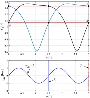
Fig. 1 Example for graphs of a dual-frequency excitation (red) and its two harmonic components as mainly used in the study (ωR1 = 3, black;ωR2 = 2, blue) with pressure amplitudes P_A1 = P_A2 = 1 bar. The vertical lines marked byT₁(black solid),T₂(blue solid) andT(red dashed) designate the periods of the high-frequency component, the low-frequency component and the dual-frequency driving, respectively.T = 3×T₁ = 2×T₂=3. (Color figure online)

4 Global Poincaré section and the period-reducing phenomenon

The parameters investigated in the present study are the pressure amplitudes (PA1,PA2) and the relative fre- quencies (ωR1, ωR2) of the dual-frequency excitation with phase shiftθ = 0, i.e.C12 = 0. The main con- trol parameters are the pressure amplitudes at several fixed frequency combinations. The ratio of each fre- quency pair is rational; therefore, periodicity of the dual-frequency driving is guaranteed (quasiperiodic forcing is excluded).

As an example, a dual-frequency excitation is pre- sented in Fig.1as a function of time together with its two periodic components atωR1=3 andωR2=2. For definiteness, the pressure amplitudes are set toPA1= PA2=1 bar. The black and blue curves are the high- and low-frequency components, respectively. Since the dimensionless timeτis defined by means of the first fre- quency component, see Eq. (5), the normalized period corresponding to the relative frequencyωR1isT1=1, indicated by the vertical black line in Fig.1. The nor- malized period of the second component (relative fre- quencyωR2) can be calculated with the frequency ratio;

that is,T2 =1/C11 =ωR1/ωR2 =3/2 = 1.5 (blue vertical line). Compare these periods with the argu- ments of the harmonic functions in equation (10) and keep in mind that the phase shift is zero (θ =C12=0).

As only normalized periods will be used throughout the article, this very often occurring quantity will be simply called “period”.

The sum of the two harmonic components results in a still periodic, but non-harmonic forcing function presented by the red curve in Fig.1. The period of this function isT = 3T1 =2T2 = 3, which is used as a global Poincaré section for the system (8)–(9). Con- sequently, during the numerical integration of the sys- tem with an initial-value problem solver, the continu- ous trajectories are sampled at time instantsτn=n·T (n = 0,1,2, . . .). Accordingly, the period, TN, of a periodic orbit is defined asTN =N ·T,N ∈ IN, and the solution is called period-Norbit. Observe, however, that in the special cases ofPA1=0 bar orPA2=0 bar, the periodT, which defines the global Poincaré section, does not coincide with the period of the actual driving T2 or T1. For PA1 = 0 bar, the dual-frequency forc- ing becomes a purely harmonic function shown by the blue curve in Fig. 1, and the continuous trajectories are sampled only after every second period of excita- tion, 2T2. Therefore, an originally period-2k solution is observed only as a period-k orbit. Similarly, when PA2 = 0 bar, the trajectories are sampled only after every third period of the excitation, 3T1(compare the black and red vertical lines in Fig.1), and the period of an originally period-3korbit is reduced from 3kto k. Thisperiod-reducing phenomenon, occurring when one of the two components of the forcing function is vanishing and only a purely harmonic excitation is left, plays an important role in the bifurcation structure of the system, discussed in more detail in Sect.5; further- more, period reduction necessarily takes place for other frequency pairs as long as the ratio of a pair is rational.

5 Results from a global scan

Throughout the following subsections, the fundamental mechanism capable of controlling multistability in har- monically driven nonlinear oscillators is presented. The basis is the period-reducing phenomenon discussed above, by which the dual-frequency treatment can gen- erate “bridges” between different periodic attractors.

First, a global picture is shown via a series of high- resolution bi-parametric plots of Lyapunov-exponent and periodicity diagrams at different frequency com- binations (the control parameters are the excitation amplitudes). Next, the details are demonstrated through a specific example with frequencies ωR1 = 3 and ωR2 = 2 (see again Fig. 1 for the driving signals).

It must be emphasized that the amplitudes for both fre- quencies of the driving can be arbitrary; that is, there

is no restriction to small-amplitude perturbations cor- responding to the second sinusoidal component.

5.1 The branching phenomenon

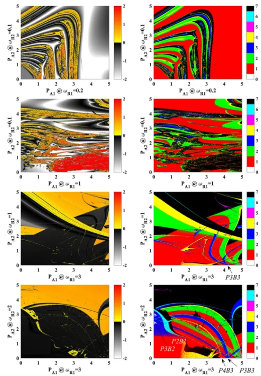
Out of the data sets for the 36 relative-frequency com- binations, four diagram pairs are shown in Fig.2at the four different relative-frequency pairs(ωR1, ωR2) = (0.2,0.1), (1,0.1), (3,1)and(3,2)organized in rows and for two different quantities (Lyapunov exponent and period) organized in columns. The left column contains the Lyapunov-exponent diagrams, where the colour-coded area means chaotic solutions (positive exponent) and where in the greyscale domains there are periodic attractors (negative exponent). In the right column, the periods of the (converged) solutions are presented up to period-6. Periodic solutions higher than six including chaos can be found in the black domains.

In the upper two rows, the plots correspond to relative frequencies lower than or equal to the linear resonance frequency (ωR1,2≤1), while the lower two rows have relative frequencies higher than or equal to the linear resonance frequency (ωR1,2≥1).

Since detailed investigations of dual-frequency driven systems for arbitrary driving amplitudes with ratio- nal frequency ratio are absent in the literature, only very few information exists about the bifurcation struc- ture shown in Fig. 2. It can be clearly seen that the dual-frequency driving causes a very complex interplay between the resonances originating from the single- frequency driven system (horizontal and vertical axes in Fig.2), see especially the first two rows of the figure.

Their comprehensive topological analysis is beyond the scope of the present study; instead, it intends to add some pieces to our knowledge by looking for special features in the diagrams. In particular, we focus on a very specific phenomenon, thebranching mechanism, turning out to be a special feature of dual-frequency driven nonlinear oscillators with rational frequency combinations, which can be used for the control of mul- tistability.

Observe that on the horizontal axis in the third row and second column of Fig.2, three period-3 branches emerge from the segment marked byP3B3(period: 3, number of the branches: 3). Similarly, three branches appear from the segmentsP4B3 andP3B3on the hor- izontal axis, and two branches are merged together at segments P2B2andP3B2 on the vertical axis in the last row and second column of Fig.2, better to be seen

Fig. 2 List of high-resolution bi-parametric plots as a function of the pressure amplitudes at different relative-frequency pairs organized in rows. Left column: Lyapunov- exponent diagrams separating the chaotic and periodic solutions. Right column: Periodicity diagrams, where periodic solutions are plotted with different colours up to period-6. Period-7 or higher solutions (including chaos) can be found in the black regions. The pressure amplitudesP_A1andP_A2are given in bar

in the enlargement and extension in Fig.3. Observe also that the number of the branches is exactly the same as the value of the corresponding relative fre- quency along the respective axis. This phenomenon will be referred to asbranching mechanismthrough- out the paper and will be investigated in more detail for the caseωR1=3, ωR2=2.

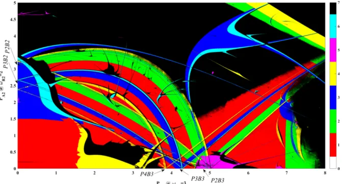
In order to get a deeper insight into the branch- ing mechanism at the relative-frequency pairωR1 = 3, ωR2 = 2, computations were repeated with much higher resolution of the pressure amplitudes (Fig.3).

The ranges of the control parameters are PA1 ∈ [0,8](bar) and PA2 ∈ [0,5](bar) with resolutions 4001 and 2501, respectively. The number of initial

Fig. 3 Bi-parametric periodicity diagram at the relative- frequency pairωR1 = 3, ωR2 = 2 with increased resolution (4001×2501) of the control parametersP_A1andP_A2. The num- ber of the initial conditions is 5×5=25 defined on an equidistant

grid in they₁–y2phase plane. The colour code is the same as in the right column of Fig.2. The pressure amplitudesP_A1andP_A2 are given in bar. (Color figure online)

conditions at a control parameter pair (PA1,PA2) is increased from 10 to 5×5=25 defined on an equidis- tant grid on they1–y2phase plane. Thus, 2501×4001×

25 ≈ 250 million initial-value problems have to be solved. This huge amount of computations is divided into 5×8 =40 (ΔPA1,2 =1 bar) segments and dis- tributed to different GPUs.

At first sight, Fig. 3 contains only slightly more information about the branching mechanism than the bottom right diagram in Fig.2, since it is hard to rep- resent the many coexisting attractors in a single plot obtained by the increased number of initial conditions (in case of coexistence, the solution with the high- est period is plotted). Investigating the system period- by-period, however, this high-resolution bi-parametric scan becomes very helpful to understand the branching mechanism (explored rigorously in the next sections);

in particular, to identify the connected branches with different periods confidently, such as the ones originat- ing fromP4B3,P3B3,P2B3,P3B2or P2B2, where, for instance,P2B3andP2B2are connected.

Typical colour combinations can be seen at the bor- der of the branch families. The three greenP2 bands are

bordered each by a yellow (period-4) band at the right border (a period-doubled zone) followed by a thin black line (indicating period-8 and higher periods including chaos that are encoded that way). Similarly, the three dark blueP3 bands are bordered each by a light blue (period-6) band, again indicating the start of a period- doubling sequence. In addition, the three yellow P4 bands are bordered by a thin black line, presumably also the beginning of a period-doubling sequence to be seen only at higher resolution. Note that also other dark blue areas are bordered on one side by a period-doubled zone of light blue followed by black. Thus, the branches themselves are period-doubling objects. It should also be noted that in any case, two of the three branches in eachPn B3,n=2,3,4, turn to the left (lower driving amplitudes PA1) and one to the right (higher driving amplitudesPA1).

5.2 Coexisting period-1 solutions

Although the red period-1 domain in Fig.3shows no sign of multiple branches, the examination of its inner

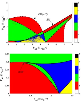
structure—the organization of the coexisting period- 1 orbits—reveals important features of the branching mechanism. They turn out to be general for other peri- ods as well. By filtering the results for period-1 orbits and by counting the number of the different attractors at a given control parameter pair, the structure of the coexisting period-1 solutions can be made visible in thePA1–PA2plane, see Fig.4with a magnification of the zone near the origin in the bottom panel. Domains with different colours represent areas with a differ- ent number of coexisting attractors up to four. These domains are bounded by saddle-node (SN, solid) and period-doubling (PD, dashed) curves computed by the boundary-value problem solver AUTO introduced in more detail later. The boundaries computed by AUTO are continuous curves. Some fractal-like shapes in the colour-coded domains are an artefact of the lack of a sufficient number of initial conditions or the presence of extremely long transients during the initial-value- problem computation Crossing one of the boundaries means the increment or decrement of the number of the attractors by one.

Multiple stable period-1 orbits in a bi-parametric space usually originate via cusp bifurcations forming pairs ofSNpoints (hysteresis) and giving rise to hys- teresis zones. The overlapping of such hysteresis zones may produce domains with a high number of coexist- ing period-1 attractors [53]. The sole cusp bifurcation in the bottom panel of Fig.4, however, cannot explain the mosaic-type pattern of the period-1 structure. The investigation of the two special cases, where one of the amplitudes of the dual-frequency driving PA1 or PA2

is zero (vertical or horizontal axis in Fig.4), can help to understand this pattern.

5.3 The limiting casePA1=0 and the period-reducing phenomenon

The bifurcation structure withPA1=0 bar is shown in Fig.5, where the first component of the Poincaré sec- tionΠ(y1)is plotted as a function ofPA2. The colour code is the same as in the cases of Fig.3and the right column of Fig. 2. For instance, red, green and blue curves are period-1, -2 and -3 orbits, respectively. Some of the periodic orbits are also marked byN×PX, where Nis the number of the coexisting attractors of periodX. The pitchfork, saddle-node and period-doubling bifur-

Fig. 4 Number of coexisting period-1 orbits in the P_A1–PA2

parameter plane at the relative-frequency pairωR1=3, ωR2= 2. The saddle-node (SN, solid) and period-doubling (PD, dashed) curves, computed by the boundary-value problem solver AUTO, are the boundaries of the domains with a different number of coexisting attractors. The pressure amplitudesP_A1andP_A2are given in bar

cation points are indicated byPF,SNandPD, respec- tively.

The period-reducing phenomenon discussed in detail in Sect.4plays an important role in the period-1 bifur- cation structure. Observe that the applied frequency combination is the same as in Fig. 1; furthermore, the first component of the dual-frequency driving is zero. Consequently, the driving is a purely harmonic function proportional to the blue curve in Fig.1, and an originally period-2k solution is observed only as period-k orbit. Thus, the first bifurcation of the sta- ble period-1 curve originating from the equilibrium solutiony1E (both amplitudes are zero) is a pitchfork pointPF, instead of a period-doubling pointPD, which gives birth of two period-1 branches 2×P1. Only the subsequent bifurcations exhibit a Feigenbaum cascade (2×P2→2×P4→ · · ·). Similarly, the first bifur- cation point in a cascade must be a symmetry-breaking bifurcation in case of a symmetric orbit in a symmetric nonlinear oscillator [54].

Fig. 5 One-dimensional bifurcation structure withP_A1=0 at the relative-frequency pairωR1 =3,ωR2 =2, where the first component of the Poincaré sectionΠ(y₁)is plotted as a function of the control parameterP_A2. The colour code is the same as in the cases of Fig.3and the right column of Fig.2. The relevant

periodic orbits are marked byN×PX, whereNis the number of the coexisting attractors of periodX. The pitchfork, saddle-node and period-doubling bifurcation points are marked byPF,SN andPD, respectively

[-]

0.6 0.7 0.8 0.9 1 1.1 1.2 1.3 1.4

y1 [-]

0 0.5 1 1.5 2 2.5 3

0 0.5 1 1.5 2 2.5 3

[-]

-2 -1 0 1 2

p A2 [bar]

R2=2 T

T2

1 1

2

2

Fig. 6 The period-reducing phenomenon. Top panel: Bubble radius versus time curvesy₁(τ)(pressure amplitudeP_A1=0 bar P_A2 = 1 bar) starting at the black dots atτ = 0 marked by the bold numbers 1 and 2 in Fig.5. Bottom panel: The sig- nal of the single-frequency driving with periodτ = T₂. The global Poincaré section applied during the present computations is defined byT(dashed, red vertical line). (Color figure online)

Two examples of bubble radius versus time curves y1(τ) are plotted in the top panel of Fig.6 so as to help understanding the period-reducing mechanism.

The blue and black period-1 solutions are initiated at PA2 = 1 bar from the black dots marked by the bold numbers 1 and 2 in Fig.5, respectively. The blue harmonic function in the bottom panel in Fig. 6 is the purely harmonic driving of the system, see also Fig. 1. It is clear that if the Poincaré sections are taken at time instancesτn = n·T (n = 0,1,2, . . .), which is used during the present simulations, the solu- tions are regarded as period-1 orbits. In contrast, if the Poincaré sections are taken at time instancesτn=n·T2

(n=0,1,2, . . .), which is a common choice in case of a purely harmonic driving, the solutions are period-2 orbits. To prevent ambiguity in the definition of the peri- odicities, solutions will be referred to as “originally”

period-N orbits if the latter definition of the Poincaré section is applied. Although the blue and black attrac- tors in Fig.6are different (each has its own basin of attraction), the only difference between them is a phase shift in time by one period of the driving (Δτ =1.5).

Altogether two types of bifurcation scenarios of periodic orbits are observable in Fig.5. For odd basic periods (period before a bifurcation cascade takes place), the first point is a pitchfork bifurcation followed by a Feigenbaum period-doubling cascade (PF →

0 1 2 3 4 5 PA2 [bar]

-0.5 0 0.5 1 1.5 2

(y2) [-]

0.15 0.2 0.25

PA2 [bar]

-0.2 -0.1 0 0.1 0.2 0.3 0.4 0.5 0.6 0.7

(y2) [-]

(A)

PD

PD

(B)

P_A1=0.6 bar SN

R1=3 R2=2 P_A1=0 bar

P_A1=0.3 bar

PF

y_2E P11

E

P12 1

P12 2 P11

E,u

P11 E+P1

2 1

PA1=0 bar ^P1₁^E,u+P1₂²

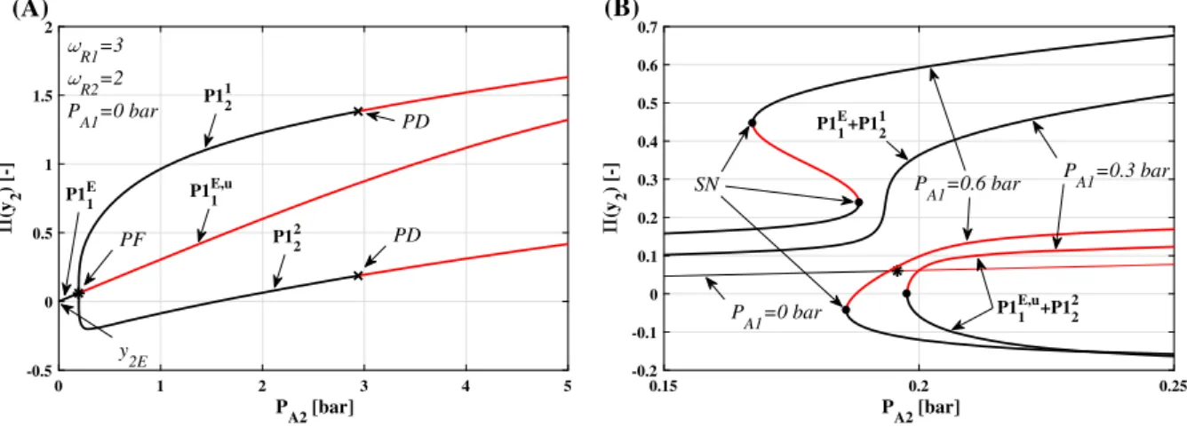
Fig. 7 Period-1 bifurcation curves computed by the boundary- value problem solver AUTO. The black and red curves are stable and unstable solutions, respectively. The asterisk, crosses and dots are the pitchfork (PF), period-doubling (PD) and saddle-

node (SN) bifurcation points, respectively. The left panel (A) shows the case with P_A1 = 0, while the right panel (B) presents results at pressure amplitude P_A1 = 0.3 bar and at P_A1=0.6 bar. (Color figure online)

PD → PD → · · ·). Some examples are the already investigated period-1 curveP1 starting from y1E, the period-3 orbits P3 originating from a SN point at PA2 =1.5 bar or the period-5 branchesP5 appearing again via aSNpoint atPA2=2 bar. Observe that the PFpoints have no influence to the colour, i.e. period.

In case of even basic periods, the period is immedi- ately halved (period-reducing phenomenon), and the bifurcation scenario is a classic Feigenbaum cascade without an initialPF point (PD → PD → · · ·). An example here is the originally period-6 solution 2×P3 generated atPA2=2.5 bar.

Through the discussion of Figs.5and6, it has been shown that the definition of the Poincaré section has an important influence on the apparent periodicity of the solutions. However, problems only appear in the two limiting cases of eitherPA1=0 bar orPA2=0 bar. In the first special case ofPA1=0 bar, a suitable choice can be eitherT2orT, see the bottom panel of Fig.6.

Since the addition of any small value to the first pres- sure amplitude PA1 will destroy the special structure introduced in Fig.5,T2will be no longer a period of the dual-frequency driving but only T. Therefore, in order to keep the definition unified, the usage ofT as a global Poincaré section is advantageous. This, at first sight only technical, extension of the definition to the limiting, purely harmonic-driving case is of great help in ordering and explaining the bifurcation scenarios of dual-frequency driven systems.

In order to illustrate this effect, it is useful to solve and compute complete bifurcation curves of periodic orbits with a boundary-value-problem solver. As an example, in Fig. 7A, the second component of the Poincaré sectionΠ(y2)of the period-1 curves is plot- ted as a function of the control parameter PA2 com- puted by the bifurcation analysis and continuation soft- ware AUTO [36]. Here, the first component of the pressure amplitude PA1is still zero. AUTO is capable of tracking down whole bifurcation curves including the unstable part even if they contain multiple turn- ing points, and it can detect the bifurcations and their types. This is the reason why AUTO is commonly used to study the bifurcation structure of nonlinear systems [5,53,55–61]. In Fig.7, the stable and unstable parts of the period-1 branches are indicated by the black and red curves, respectively. The curve originating from y2E becomes unstable via a pitchfork bifurcationPF at PA2 = 0.19 bar producing two stable coexisting period-1 branches. These stable curves lose their stabil- ity approximately atPA2=3 bar by a period-doubling pointPD.

5.4 Perturbation of the limiting casePA1=0

The breakup of the structurally unstable pitchfork bifur- cation due to the effect of a nonzero value of the ampli- tude of the first harmonic component of the excitation (PA1=0.3 bar) is clearly seen in Fig.7B. The curves marked byP1₁^EandP1¹₂in Fig.7A form a single curve

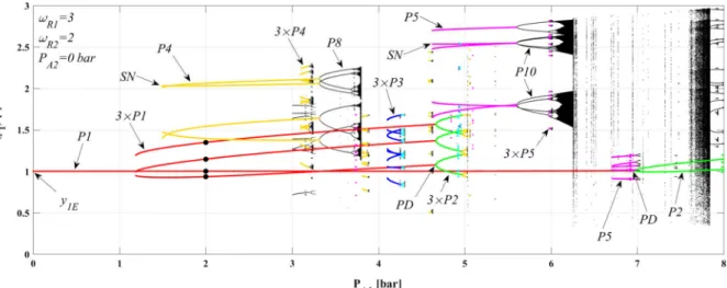
Fig. 8 One-dimensional bifurcation structure withP_A2=0 at the relative-frequency pairωR1 =3,ωR2 =2, where the first component of the Poincaré sectionΠ(y₁)is plotted as a function of the control parameterP_A1. The colour code is the same as in the cases of Fig.3and the right column of Fig.2. The relevant

periodic orbits are marked byN×PX, whereN is the number of the coexisting attractors of periodX. The saddle-node and period-doubling bifurcation points are marked bySNandPD, respectively. (Color figure online)

P1₁^E+P1¹₂in Fig.7B. Likewise, the curvesP1₁^E,uand P1²₂ presented in Fig.7A form again a single curve P1₁^E,u+P1²₂in Fig.7B composed by a stable and an unstable part separated by a saddle-node bifurcation (black dot) at the turning point. Elevating PA1 from 0.3 bar to 0.6 bar, a pair ofSNpoints appears along the branchP1₁^E+P1¹₂forming a hysteresis. Observe that both curves P1₁^E +P1¹₂andP1₁^E,u+P1²₂have their own separate evolution as the amplitudePA1changes;

consequently, the black and blue curves in the top of Fig.6must become different (not only by a phase shift in time) forPA1>0 bar as they have their own sepa- rate evolution as well. All the pitchfork structures in the bifurcation scenarios initiated from odd basic periods are broken up in the same way as presented in Fig.7B, except for the formation of the hysteresis which not necessarily happens.

5.5 The limiting casePA2=0

Shortly in this section, the complex development of the period-1 structure in a wide range of the amplitudes PA1andPA2will be discussed in detail. Up to now, it is important only to understand how the period-reducing mechanism works for single-frequency driving, how it decomposes periodic solutions into multiple orbits of

lower periodicities, and how these multiple orbits are separated under the perturbation of the amplitude of the other harmonic component. In order to understand the global picture, however, the investigation of the other special case, where the control parameter is PA1and the amplitude of the second component PA2 is zero, is necessary. The corresponding bifurcation diagram is shown in Fig.8, where the first component of the Poincaré sectionΠ(y1)is plotted as a function of the pressure amplitudePA1. The colour code and the nota- tion system are the same as in Fig.5. At first sight—in view of (2) withθ = 0—both cases (PA1 = 0 and PA1=0) seem exchangeable. However, switching to the other frequency component, different bifurcation scenarios develop (if the frequencies are distinct).

There are two types of bifurcation scenarios of peri- odic orbits. If the basic (original) period is divisible by 3, then the period reducing takes place immediately decreasing the period of the orbits from 3ktokfollowed by a Feigenbaum cascade as usual (PD→PD→ · · ·).

Notable examples are the branches 3×P1 and 3×P3 both appearing viaSNbifurcations at PA1 = 1.2 bar and at PA1 = 4.1 bar, respectively. For other basic periods, there is no period-reducing phenomenon, but only a period-doubling cascade. Examples of this sce- nario are the period-1 curve departing from the equi- librium solutiony1E, the period-4 orbits generated at

0 0.5 1 1.5 2 2.5 3 [-]

0.6 0.7 0.8 0.9 1 1.1 1.2 1.3 1.4

y1 [-]

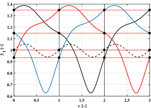
Fig. 9 The period-reducing phenomenon. Dimensionless bub- ble radius versus time curves of four coexisting stable period-1 orbits at pressure amplitudeP_A1=2 bar starting from the black dots shown in Fig.8atτ=0. Between the black, red and blue solid curves there is only a phase shift in time withΔτ = 1 or 2. The dashed curve is a degenerate (i.e. repeating only after T₁instead of afterT), small-bubble-radius-amplitude case that exists stably up to P_A1 ≈ 7 bar where the oscillation period doubles. (Color figure online)

PA1 = 1.5 bar or the period-5 branches initiated at PA1 =4.6 bar. Observe that there are no pitchfork or other special bifurcations present in these cases.

Figure8explains how the coexistence is possible of altogether four period-1 stable solutions highlighted in Fig.4 by the yellow domain. The period-1 orbit P1 emerges from the equilibrium point y1E and remains

stable up to the pressure amplitude PA1 ≈ 7 bar. It loses its stability there via a period-doubling bifur- cation. The originally period-3 family of solutions 3×P1 appearing through aSNpoint is decoupled into three period-1 branches existing between the ampli- tudesPA1≈1.19 bar andPA1≈4.67 bar. Therefore, there is a wide range of amplitudes PA1 where four period-1 attractors exist. Figure9shows these coexist- ing orbits at PA1 =2 bar starting from the black dots in Fig.8. The dashed curve is the period-1 orbit related to the curve originating fromy1E. The black, red and blue solid curves are the orbits of the period-reduced 3×P1 branches, where the only difference between them is again a phase shift in time, in this case of one or two periodsT1(Δτ =1 or 2).

5.6 Perturbation of the limiting casePA2=0

Again, the boundary-value-problem solver AUTO can help to understand the behaviour of the system under a small perturbation of the amplitude of the second, harmonic component of the driving (PA2 > 0). The bifurcation curves related to the four period-1 orbits can be seen in Fig.10A for PA2 = 0 bar. The black and red curves mean stable and unstable orbits, respec- tively. The bifurcation of the saddle-node (SN) and period-doubling (PD) points are also detected. They are marked by dots (SN) and crosses (PD). Observe

0 1 2 3 4 5 6 7 8

PA1 [bar]

-0.5 0 0.5 1 1.5 2 2.5

(y2) [-]

0.5 1 1.5 2

PA1 [bar]

-0.4 -0.2 0 0.2 0.4 0.6 0.8 1 1.2 1.4

(y2) [-]

SN

PD

(A) (B)

R1=3 R2=2 P_A2=0 bar

P_A2=0.1 bar

y_2E P11

E

P13 1

P13 3

P13 2

Fig. 10 Period-1 bifurcation curves computed by the boundary- value problem solver AUTO. The black and red curves are stable and unstable solutions, respectively. The crosses and dots are the period-doubling (PD) and saddle-node (SN) bifurcation points, respectively. The left panel (A) shows the case withP_A2=0,

while the right panel (B) presents results of the 3×P1 curves at the pressure amplitude ofP_A2=0.1 bar. The arrows in panel (B) show the motion of theSNbifurcation points, two of them towards lowerP_A1, one of them towards largerP_A1. (Color figure online)

that the PA1-ranges of the stable (black) segments in Fig.10A coincide with the domain of existence of the corresponding parts of the red curves in Fig.8. On the right hand side of Fig.10, only the evolution of the curves 3×P1 is presented by increasing the ampli- tudePA2from zero to 0.1 bar. It is clear that while the saddle-node bifurcations (black dots) take place at the same value ofPA1when PA2=0 bar (see the vertical thin line in Fig.10B), the locations of these bifurcation points differ whenPA2 >0. This means that each of the three bifurcation curves have their own evolution as the amplitudePA2changes. Consequently, the black, red and blue solid curves in Fig.9become different (not only by a phase shift in time) forPA2>0.

6 Period 1: the complete picture

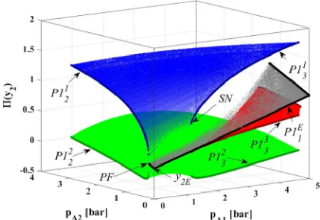
Due to the exhaustive discussion in the preceding sec- tions, it is clear now how the system behaves under single-frequency driving when a second, harmonic component is added as a perturbation. The huge amount of results presented in Fig.3 can help to establish a global overview of the evolution of all the period-1 solutions by means of filtering the results by period, here period-1. Figure11 shows these period-1 solu- tions represented in a three-dimensional plot, where the second component of the Poincaré section,Π(y2), the bubble wall velocity, is plotted as a function of the two main control parameters PA1 and PA2. The different period-1 orbits can be decomposed into several layers indicated by the blue, black, red and green surfaces.

In the limit cases when one of the pressure amplitudes is zero (planesΠ(y2)–PA1orΠ(y2)–PA2), the points are plotted with bigger markers to be able to distin- guish such special solutions more easily. These solu- tions, which form complete bifurcations curves pre- sented in Figs.7A and10A, are marked byP1^m_n, where n is the original period andm = 1, . . . ,n is a serial number,P1 means period-1 solution. When bothPA1

andPA2are zero then the system is in equilibrium and the dimensionless bubble wall velocity and its Poincaré section y2E are zero (it is the origin of the diagram).

The black period-1 surface originating from this point is marked byP1₁^E(instead ofP1¹₁, emphasizing the equi- librium originE). There is only one curve of this type, which is a surface of small-amplitude bubble oscilla- tions.

Fig. 11 3D representation of the stable period-1 orbits (Poincaré section points of the bubble wall velocity) above the parameter planeP_A1–PA2 by filtering the results presented in Fig.3by period, here period-1. The period-1 orbits can be separated into four different layers marked by the blue, black, red and green surfaces. The indication of the curves in theΠ(y₂)–PA1(Fig.10) orΠ(y₂)–P_A2(Fig.7) planes is P1^m_n, wherenis the original period andm=1, . . . ,nis a serial number,P1 means period- 1 solution. The black surface originating from the equilibrium solution of the system is marked by P1₁^E (instead ofP1¹₁to show the connection with the equilibrium point). (Color figure online)

Figure11indicates a very interesting phenomenon, namely the originally period-2 solutions on P1¹₂can be transformed into the originally period-3 solutions on P1¹₃through the blue surface. Similarly, orbits on P1²₂ can be transformed into orbits on P1²₃ via the green surface. These are smooth transformations by means of the continuous change of the amplitudesPA1

and PA2 of the dual-frequency driving. Naturally, all these orbits are considered as period-1 attractors due to the specific choice of the global Poincaré section.

Consider, however, the following scenario of parame- ter variations visualized by the supplementary movie file (Online Resource 1) where the top panel shows the dimensionless bubble radius curvesy1as a function of the dimensionless timeτ, and the bottom panel repre- sents the dual-frequency driving signalPA(τ)(exclud- ing the static ambient pressure).

Firstly, let us start the investigation with a solu- tion lying on the bifurcation curve 2× P1 in Fig. 5 (P1¹₂ or P1²₂ in Fig. 11) so that the amplitude of the single-frequency excitation is somewhere between PA2=1.4 bar and PA2=2.9 bar (PA1=0 bar) with relative frequency ωR2 = 2. Specifically, in Online Resource 1, the pressure amplitude is chosen to be P = 2.5 bar. In this video, besides the originally