Endogenous choice of decision variables
Attila Tasn´adi∗
MTA-BCE “Lend¨ulet” Strategic Interactions Research Group, Department of Mathematics, Corvinus University of Budapest†
June 4, 2012
Abstract
In this paper we allow the firms to choose their prices and quantities simultaneously.
Quantities are produced in advance and their common sales price is determined by the market. Firms offer their “residual capacities” at their announced prices and the corresponding demand will be served to order. If all firms have small capacities, we obtain the Bertrand solution; while if at least one firm has a sufficiently large capacity, the Cournot outcome and a model of price leadership could emerge.
Mathematics Subject Classification (2010):91A40
Journal of Economic Literature Classification: D43, L13.
Keywords:Cournot, Bertrand-Edgeworth, Price Leadership.
1 Introduction
We consider a game in which the firms simultaneously choose their price and quantity decisions. This work complements Tasn´adi (2006 and 2010) in which firms could choose their decision variable (price or quantity). In Tasn´adi (2006) the firms chose between price and quantity, and second, they selected their prices or quantities with respect to their first-round decisions. Given the firms’ first-stage decisions the price setters, if there were at least two of them, had to play mixed strategies like in the capacity-constrained Bertrand- Edgeworth game. Therefore, we had to limit ourselves to the case of symmetric capacities for which we found under reasonable assumptions the emergences of the Cournot game. In Chapter 5 of Tasn´adi (2010) we considered the case in which the firms must choose their decision variables and their magnitudes simultaneously, by which approach we could avoid the problem of dealing with mixed strategies, and therefore, we could also investigate the case of asymmetric capacities. We found that for a large region of capacity constraints both the Cournot and the Forchheimer outcome could arise.
In contrast to the above mentioned two works, in which the firms had to make a binary choice, we allow in this paper the firms to make a smooth decision. The two extreme cases of
∗Financial support from the Hungarian Scientific Research Fund (OTKA K-101224) is gratefully ac- knowledged.
†F˝ov´am t´er 8, 1093 Budapest, Hungary (e-mail: attila.tasnadi@uni-corvinus.hu)
setting zero quantity or setting a sufficiently large price would give us a purely price-setting firm and a purely quantity-setting firm, respectively. In particular, firms can produce a quantity for which the market determines price by equating supply and demand, and firms can choose the price for their additional production. In the interesting range of capacities we find the emergence of the Cournot and the Forchheimer outcome.
The endogenous choice of decision variables has been investigated in the literature for homogeneous good oligopoly markets by Dastidar (1996) and Qin and Stuart (1997).
Dastidar (1996) considered a two-stage duopoly game in which the firms choose their decision variables in stage 1 and the magnitude of the selected decision variable in stage 2. In case of two quantity setters a Cournot duopoly game is played in stage 2, in case of two price setters a Bertrand duopoly game is played in stage 2, while in case of one price-setter and one quantity setter we have that the quantity setter takes the price set by the price setter as given. Dastidar (1996) finds that a mixed equilibrium never occurs, the Cournot game always emerges as an equilibrium, while the Bertrand game may emerge as the outcome of the two-stage game. Qin and Stuart (1997) formulated an oligopoly game in which some firms set their quantities and the remaining firms set their prices. They showed that if the firms are free to choose their decision variable, then both the Bertrand and the Cournot outcome could emerge. Tasn´adi (2006 and 2010) and this paper considers Bertrand-Edgeworth-type price-setting instead of Bertrand-type price-setting behavior.
For more on the role of decision variables in the homogeneous good framework we refer to Friedman (1988).
The seminal paper allowing the duopolists to choose their decision variable, is due to Singh and Vives (1984) that investigates a heterogeneous goods two-stage duopoly market.
Singh and Vives (1984) demonstrated the emergence of the Cournot game if goods are substitutes and the emergence of the Bertrand game if goods are complements. Klemperer and Meyer (1986) investigates a one-stage heterogeneous goods duopoly game and reports that a multiplicity of equilibria is possible. For more on the endogenous choice of the decision variable in the heterogeneous goods framework see, for instance, Szidarovszky and Moln´ar (1992), Tanaka (2001a and 2001b) and Reisinger and Ressner (2009), among others.
The remainder of the paper is organized as follows. Section 2 presents our framework.
Section 3 contains our analysis. Finally, we conclude in Section 4.
2 Framework
Suppose that there are n firms on the market, where we shall denote the set of firms by N ={1, . . . , n}. We assume that the firms have zero unit costs.1 We shall denote bykithe capacity constraint of firmiand byK =Pn
i=1ki the aggregate capacity of the firms. Let the capacity constraints be ordered decreasingly, that isk1 ≥. . .≥kn>0. We summarize the assumptions imposed on the oligopolists’ cost functions below:
Assumption 1. There are n firms on the market with zero unit costs and capacity constraints k1 ≥k2≥. . .≥kn>0.
The demand is given by functionD on which we impose the following restrictions:
1Since the firms, which set also prices, basically compete in a residual production-to-order game (that is, production takes place after the firms’ prices are revealed), the real assumption here is that the firms have identical unit costs.
Assumption 2. The demand function Dintersects the horizontal axis at quantityaand the vertical axis at price b. D is strictly decreasing and twice continuously differentiable on (0, a); moreover, D is right-continuous at 0, left-continuous at b and D(p) = 0 for all p≥b.
Clearly, a price-setting firm will not set its price above b. Let us denote by P the inverse demand function. Thus, P(q) = D−1(q) for 0< q ≤a, P(0) =b, and P(q) = 0 forq > a. In addition, we shall denote bypc the market clearing price, i.e. pc=P(K).
The following technical assumption is needed to ensure the existence of an equilibrium in our model.
Assumption 3. The functionpD0(p) +D(p) is strictly decreasing on (0, b).
We shall denote byDri (p) = (D(p)−(K−ki))+ the residual demand curve of firm i and its inverse byPir(q). It can be easily verified thatPir(q) =P(q+ (K−ki)). Assuming efficient rationing, the function πri (p) =pDri (p) will equal firm i’s profit whenever it sets the highest price in the pure price-setting game and p ≥ pc. We ensure that every firm will be active in the market by the next assumption.
Assumption 4. We assume thatK−kn< a.
We shall denote by pmi the unique revenue maximizing price on the residual demand curveDirand byqimthe unique revenue maximizing output on the inverse residual demand curvePir, i.e.pmi = arg maxp∈[0,b]pDri (p) andqim= arg maxq∈[0,a]qPir(q) for anyi∈N. Of course, qim =Dir(pmi ). Furthermore, it can be checked that pm1 ≥pm2 ≥. . .≥pmn because of Assumptions 1-4. Let πi = πri (pmi ). Clearly, pc and pmi are well defined whenever Assumptions 1-4 are satisfied. Note that Assumption 4 also ensures that pmi > 0 and πi >0.
Let pi ∈ [0, b] be the price and qi ∈ [0, ki] be the quantity decision of firm i ∈ N. Hence, the price decisions and the quantity decisions are contained in vectors p ∈[0, b]n and q∈ ×nj=1[0, kj], respectively. If firm isets a positive quantity qi, then it will sell this amount at a price determined by the market. Furthermore, if firmisets its pricepi below b, then it is willing to produce in addition an amount of at most ki−qi units at pricepi, which we shall call the residual capacity of firm i. We to refer to firm i as a pure price setter if pi < band qi = 0 and as a pure quantity setter ifpi=b and qi >0. Otherwise, a firm is a price and quantity setter at the same time. We denote byJp,q={j∈N |qj >0}
the set of quantity-setting firms and by Ip,q = N \Jp,q the set of purely price-setting firms. For fixed decisions (p,q) the aggregate supply of the firms at price p is given by Sp,q(p) =P
i∈Nqj+P
i∈N,pi≤p(ki−qi).
We have to specify a demand-allocating mechanism and the price of the quantity- setting firms’ product as a function of the price and quantity actions taken by the firms.
We define the quantity-setting firms’ sales price, denoted by p∗(p,q), to be the lowest price at which the demand is less or equal to the aggregate supply of the firms. Formally, p∗(p,q) =
inf{p∈[0, b]|D(p)≤Sp,q(p)}= min{p∈[0, b]|D(p)≤Sp,q(p)}.
We can write min instead of inf becauseD(p)−Sp,q(p) is a decreasing and right-continuous function inp. Observe thatp∗(p,q) is even defined in case ofIp,q=N.
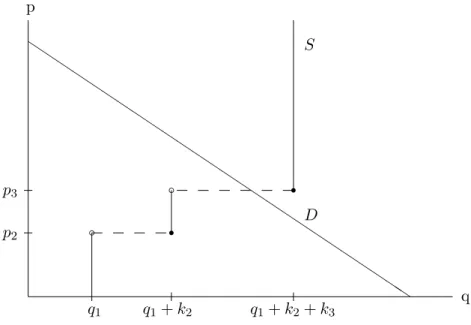
At price level p∗(p,q) aggregate supply may exceed market demand. This case is illustrated in Figure 1 in which there are two price-setting firms and one quantity-setting
p
q Q
Q Q
Q Q
Q Q
Q Q
Q Q
Q Q
Q Q
Q Q
Q Q
Q Q
Q Q
Q QQ S
D p2
p3
b
q1
r b
q1+k2
r
q1+k2+k3
Figure 1: Quantity-setting firms product price
firm. In the situation presented in Figure 1 the sales price for the quantity-setting firm’s product equals p3 (where p1 = b and q2 = q3 = 0). In case of price ties, we assume for simplicity, that the demand is allocated first to the quantity-setting firms and afterwards the remaining demand is shared by the price-setting firms in proportion of their capacities.
The first part of this assumption, i.e. that the demand is allocated first to the quantity- setting firms, expresses our intuition that price setters shall face quantity adjustment, while quantity setters shall face price adjustment. The demand satisfied by firm j ∈Jp,q
at pricep∗(p,q) is given by
∆qj(p,q) =
( qj if p∗(p,q)>0, min
n qj,Pnqj
l=1qlD(0) o
if p∗(p,q) = 0;
and therefore, its profit equals πjq(p,q) = p∗(p,q)qj from producing quantity qj. In addition, let πqi (p,q) = 0 for any i∈Ip,q. We define the demand satisfied by firmi∈N resulting from its price-setting activity by
∆pi(p,q) =
0 if pi> p∗(p,q) orqi=ki,
ki−qi P
pl=pikl−ql
D(pi)−Pn
j=1qj−P
pl<pi(kl−ql)+
if pi=p∗(p,q) andqi< ki,
ki−qi if pi< p∗(p,q) andqi< ki.
Thus, firm i∈N makesπpi (p,q) =pi∆pi(p,q) profit from selling its residual capacity at pricepi. Finally, we shall define the profit of firmi∈N byπi(p,q) =πip(p,q) +πiq(p,q).
3 The analysis
In this Section we determine those conditions under which an equilibrium in pure strategies exists. We will proceed step by step in order to obtain a better understanding of the equilibrium behavior of our oligopoly game. The following Lemma states that in a pure- strategy equilibrium the purely price-setting firms must set the same prices.
Lemma 1. Under Assumptions 1-4, if (p,q) is a pure-strategy equilibrium, then pi =pj for any i, j∈Ip,q.
Proof. The statement is obviously true if |Ip,q| ≤ 1. Thus, we have only to consider the case of |Ip,q|>1. Let firm j be one of the firms setting the lowest price; that is, pj ≤pi
for alli∈Ip,q. Suppose thatpj < pi holds for a firm i∈Ip,q. If ∆pi(p,q)>0, then firmj can increase its profit by setting its price arbitrarily close to but belowpi. If ∆pi (p,q) = 0, thenπi(p,q) = 0. But firmican make positive profit, for instance, by switching its price toP 12(K−ki+a)
so that it faces a positive demand because of Assumption 4. Thus, firm iwould deviate, and therefore,pj < pi cannot be the case.
Next, we prove that in a pure-strategy equilibrium every purely price-setting firm’s price must be equal to the sales price of the quantity-setting firms.
Lemma 2. Let Assumptions 1-4 be satisfied and (p,q) be a pure-strategy equilibrium. If
|Jp,q|>0, then pi =p∗(p,q) for any i∈Ip,q.
Proof. Clearly, the Lemma holds if |Ip,q|= 0. Therefore, in what follows we can assume that|Ip,q|>0. Suppose thatpi 6=p∗(p,q) for somei∈Ip,q. Recall that any firmi∈Ip,q
setting its price below p∗(p,q) can sell its entire capacity ki. Moreover, observe that p∗(p,q) will not change if prices lower thanp∗(p,q) change as long as they remain lower thanp∗(p,q). Thus, ifpi< p∗(p,q), firmican increase its profit by setting a price slightly below p∗(p,q), since it is still selling ki but at a higher price. If pi > p∗(p,q), then firm i does not sell anything and makes zero profit. But firm i can achieve positive profit by making a sufficiently large price reduction because of Assumption 4; a contradiction.
Furthermore, if the equilibrium market price is larger than the market-clearing price and there is at least one purely price-setting firm in the market, then in a pure-strategy equilibrium the quantity-setting firms produce at their capacity limits, and thus there are no “partially” price-setting firms in the market.
Lemma 3. Let Assumptions 1-4 be satisfied and (p,q) be a pure-strategy equilibrium. If
|Jp,q|>0,|Ip,q|>0 and p∗(p,q)> pc, then we must have qj =kj for all j ∈Jp,q in any pure-strategy equilibrium.
Proof. From Lemma 2 we know that in a pure-strategy equilibrium pi = p∗(p,q) must hold for alli∈Ip,q. Moreover, every firm’s profit must be positive because of Assumption 4, which implies ∆pi (p,q)>0 for anyi∈Ip,q and ∆qj(p,q)>0 for anyj ∈Jp,q.
Suppose that qj < kj for a firm j ∈Jp,q. Then we have to distinguish the following three cases: (i) pj < p∗(p,q), (ii) pj = p∗(p,q) and (iii) pj > p∗(p,q). In case (i) firm j can increase its profit by increasing its output to kj because this will not decrease p∗(p,q), since its previously sold kj −qj units can be now sold at price p∗(p,q). In case (ii) a purely price-setting firm could capture market from j by unilaterally undercutting price pj.2 Finally, in case (iii) firm j selling a positive amount at price pj would be in contradiction with the definition ofp∗(p,q). Hence, quantity-setting firmj could increase its profits by increasing its quantity since this would just result in a decrease of sales for the purely price-setting firms. We obtained in any of the three cases a contradiction, and therefore we must haveqj =kj in any pure-strategy equilibrium with an equilibrium price larger than the market-clearing price.
2At this point we are employingp∗(p,q)> pc.
Now we are ready to prove the main propositions considering our oligopoly game.
The next proposition establishes that the Bertrand solution is the only possible Nash equilibrium candidate in the presence of at least two purely price-setting firms.
Proposition 1. Let Assumptions 1-4 be satisfied and(p,q)be a pure-strategy equilibrium.
If |Ip,q| ≥2, then the only possible pure-strategy Nash equilibrium candidate isqj =kj or pj =pc for all j∈Jp,q andpi=pc for alli∈Ip,q.
Proof. Suppose that |Jp,q| = 0. By Lemma 1 we know that in a possible equilibrium every purely price-setting firm sets the same price. But, if that price level exceedspc, then their sales will be less than their capacity level, and therefore, any of them can gain from undercutting its opponents.
Now, we consider case |Jp,q| > 0. By Lemma 2 we must have pi = p∗(p,q) for any i∈Ip,q. Of course,pc≤p∗(p,q). Suppose thatpc< p∗(p,q). Then we know by Lemma 3 that qj =kj for allj ∈Jp,q. But ifpc< p∗(p,q), then any price-setting firmi∈Ip,q will sell less thanki products. Therefore, by just unilaterally undercutting pricep∗(p,q), any price-setting firm can increase its sales radically, and thus, increase its profits. Hence, in an equilibrium we must havepc=p∗(p,q) and only strategy profiles specified by Proposition 1 remain.
Ifki≤qmi , then we will say that firmi∈N hasscarce capacity, while otherwise we will say that firm i∈N hassufficient capacity. Note that a firm with scarce capacity will be eager to produce at its capacity limit. We shall denote by H the set of those firms having only scarce capacity, i.e.H ={i∈N |ki ≤qim}. It can be verified that conditionki ≤qim is equivalent topc≥pmi . Thus,H ={i∈N |h≤i≤n}for someh∈ {1, . . . , n+ 1}since the sequencepmi is nonincreasing.
In the following proposition we establish that the Bertrand solution is the unique Nash equilibrium solution in pure strategies of any mixed oligopoly game if every firm has scarce capacity.
Proposition 2. Under Assumptions 1-4, if H =N and (p,q) is an equilibrium in pure strategies, then it must be payoff and price equivalent with the Bertrand solution, i.e. the equilibrium price equals the market-clearing price and all firms sell their entire capacity.
Proof. We can verify thatqj =kj orpj =pc for anyj∈Jp,q and pi =pc for anyi∈Ip,q is a Nash equilibrium because of Assumptions 2, 3 and ki ≤qim for all i∈N.
Assume that|Ip,q|= 0. Then the partial price setter selecting the highest price above pc would reduce its price because of pmi ≥pc. In addition, if there are more partial price setters choosing the same highest price above pc, then each of them could benefit from a slight price reduction. Hence, only profiles specified in Proposition 2 can be equilibrium profiles.
We turn to the analysis of caseIp,q={i}. Suppose thatpc< p∗(p,q). Then by Lemma 3 each quantity-setting firmj∈Jp,qsetsqj =kj and by Lemma 2 the purely price-setting firm ishould set price pi =p∗(p,q). Since by pc≥pmi firm ihas an incentive for a price reductionpc< p∗(p,q) cannot be the case in an equilibrium. Again, only profiles specified in Proposition 2 can be equilibrium profiles.
Finally, if |Ip,q| ≥2, then Proposition 1 yields the desired result.
Let us denote by pdi the smallest price satisfying pdi min{ki, D pdi
} = pmi Dri (pmi ).
Suppose that firm i has sufficient capacity (implying pdi < pmi ), then firm iis indifferent
to whether serving residual demand at price level pmi or selling its entire capacity at the lower price level pdi. We will need the following Lemma established for the two firm case by Deneckere and Kovenock (1992) and for the nfirm case by (Tasn´adi 2010, Lemma 7).
Lemma 4. Suppose that firm iand j have both sufficient capacity and that Assumptions 1-4 are satisfied. If i < j, then pdi ≥pdj. In addition, if ki > kj, then pdi > pdj.
Next, we investigate the case of only one purely price-setting firm. Because of Propo- sition 2 we may assume in what follows that there is a firm having sufficient capacity.
Proposition 3. Under Assumptions 1-4, if(p,q)is an equilibrium in pure strategies such that Ip,q={i} ⊂N\H ={1, . . . , h−1} then the equilibrium is given by
∀j∈Jp,q:qj =kj and pi =pmi = arg max
p∈[0,b]pDir(p). (1)
In addition, the above type of equilibrium exists if and only if pd1 ≤pmi .
Proof. First, we demonstrate that ifpd1 ≤pmi , then the strategy profile given by equation (1) is an equilibrium. Suppose that a quantity-setting firm chooses a strategy (pj, qj) different from (b, kj). Clearly, firmjwould reduce its profits by selling its residual capacity at a pricepj < pmi . Ifpj > pmi , then it can sellq0j =
D(p)−qj−P
l6=jkl
+
units at price pj, which means that firmj faces its residual demand curve. Hence, firmj would be better off by selling kj units at price pmi because of pdj ≤ pd1 ≤ pmi . For quantity-setting firm j the case of pj = pmi remains to be investigated. In the latter case a unilateral output decrease from ki to at most qim will not change the sales price for the quantity-setting firms’ product, but only increase the purely price-setting firm’s sales. Moreover, if firm j reduces its output below qim, then the sales price for the quantity-setting firms’ product will equal to Pjr
qj+P
l6=jkl
. Thus, a unilateral output decrease by any firm j ∈Jp,q
withj > iwill inevitably lead to a decrease in its own profit level because ofpmj ≤pmi and Assumptions 2 and 4. Furthermore, an output reduction by firm j∈Jp,q with j < i will increase its profits if and only if pdj > pmi , because then a decrease in output to qjm yields pdjkj profits, which is greater thanpmi kj. Regarding that the sequencepdj is nonincreasing, we have shown that the quantity-setting firms will not deviate from qj = kj. It can be easily checked that firmiwill not deviate from pricepmi . Hence, equation (1) determines a Nash equilibrium profile, which determines the set of equilibrium profiles in the presence of one purely price-setting firm because of Lemmas 2 and 3.
Second, we establish that if pd1 > pmi , then there is a lack of Nash equilibrium with one purely price-setting firm. We already know by Lemmas 2 and 3 that in an equilibrium qj =kj for all j ∈Jp,q and pi =p∗(p,q) must hold. Therefore, price-setting firm i sets pricepmi and sellsqim amount of product. This means thatpi =pc(p,q) must be equal to pmi in a Nash equilibrium. But, then firm 1 will unilaterally decrease its outputs, because pm1 qm1 =pd1k1 > pmi k1 and we conclude that a Nash equilibrium does not exist.
Checking the proof of Proposition 3, we obtain the following Corollary.
Corollary 1. Let Assumptions 1-4 and pd1 ≤ pmi be satisfied, and let i ∈ N \H = {1, . . . , h−1}. Then
∀j∈N\ {i}:qj =kj , qi∈[0, qim]and pi =pmi = arg max
p∈[0,b]pDir(p) (2) determines all equilibria with one partial or pure price-setting firm.
We have to emphasize that by Proposition 3 our oligopoly game, with a price-setting firmihaving sufficient capacity and fulfilling conditionpd1 ≤pmi , yields an implementation of Forchheimer’s model of dominant firm price leadership, because the price-setting firm sets its price by maximizing profits with respect to its residual demand curve and the sales price for the remaining firms’ product equals that price. Let us remark that, to act as a price leader, a firm does not have to possess the largest capacity on the market so far the requirements of Proposition 3 are satisfied. For more on price leadership we refer to Ono (1982), Deneckere and Kovenock (1992), van Damme and Hurkens (2004), Tasn´adi (2004) or Yano and Komatsubara (2006).
We still have to consider the Cournot game, that is the case in which every firm behaves as a pure quantity setter. The existence of a Nash equilibrium in the Cournot game has been investigated extensively in the literature (see for instance Szidarovszky and Yakowitz, 1977; Novshek, 1985; Amir, 1996; Forg´o, 1996). Regarding our assumptions, the results known to us cannot be applied directly to demonstrate existence in our model. Particularly, we assume that the function pD(p) is strictly concave, which does not even imply that qP (q) is concave. To verify this consider demand functionD(p) = 1−43p3/4, which satisfies Assumption 2 and 3, but for which qP(q) is convex in the interval (6/7,1). Moreover, it can be verified that the concavity ofpD(p) does not even imply the log-concavity ofP(q).
Hence, even Amir’s (1996) existence theorem cannot be applied. However, we will prove the existence of a Nash equilibrium by applying Debreu’s (1952) existence theorem.
Proposition 4. Under Assumptions 1-4, the Cournot game has an equilibrium in pure strategies.
Proof. Firm i’s strategy set [0, ki] is compact and its payoff function qi P P
j∈Nqj is continuous. In order to apply Debreu’s (1952) existence theorem we still have to show that the firms’ payoff functions are quasiconcave in their own decision variable. We will demonstrate that Πi(qi, Q−i) =qiP(qi+Q−i) is single peaked inqi for any fixed value of Q−i ∈[0, K−ki], which in turn implies quasiconcavity.
Pick an arbitrary value for Q−i from interval [0, K−ki]. Let us define the function F : [0, a−Q−i] → [0, c] by F(q) =P(q+Q−i), where c= P(Q−i). We shall denote by G the inverse function of F. It can be checked that G(p) = D(p)−Q−i. Let Π∗i (p) = p(D(p)−Q−i)+. Of course, Π∗i (0) = 0, Π∗i (p) = 0 for any p ≥ c, and Π∗i is strictly concave in (0, c). Hence, it has a unique maximum, denoted by p∗ ∈(0, c), which can be determined by the following equation:
d
dpΠ∗i (p) =G(p) +pG0(p) = 0 (3) The first-order condition corresponding to problem maxqiΠi(qi, Q−i) is
d
dqΠi(q, Q−i) =F(q) +qF0(q) = 0. (4) We check that q∗ =G(p∗) satisfies equation (4):
d
dqΠi(q∗, Q−i) =F(q∗) +q∗F0(q∗) =p∗+G(p∗) 1
G0(p∗) = 0,
where the last equality holds clearly becausep∗is a solution of equation (3) andG0(p∗)6= 0.
Furthermore, q∗ is the unique solution of equation (4) since otherwise equation (3) will not have a unique solution. Finally, output level q∗ corresponds to a maximum since Πi(q∗, Q−i)>0 and Πi(0, Q−i) = Πi(a−Q−i, Q−i) = 0.
The next theorem summarizes our results concerning our oligopoly game:
Theorem 1. Under Assumptions 1-4 the following statements hold true concerning our oligopoly game:
1. Ifqmi ≥ki for all i∈N, then any Nash equilibrium yields the Bertrand solution.
2. If i < h and pd1 ≤pmi , then the second type of equilibria result in a model of price leadership.
3. If there exists an i∈N such that qmi < ki, then third type of equilibria are given by the Cournot solutions.
4. Another type of Nash equilibrium does not exist.
Proof. Points 1 and 2 follow from Proposition 2 and Corollary 1.
Next, we show point 3, that is (p, yi) for all i ∈ N is a Nash equilibrium, where y denotes a Cournot solution andp≥p∗ =P(Pn
i=1yi). Suppose that firmi∈N considers to become a pure or partial price setter, and thus switches to another strategy (pi, qi)6= (p, yi).
Since in any case firmifaces residual demand curve
D(pi)−qi−P
j6=iyj
+
as a partial (qi >0) or pure (qi= 0) price setter it can be easily verified that (p, yi) is a best response to the other firms strategies.
Finally, point 4 follows from our established facts that the presence of at least one pure price setter implies that there cannot be a partial price setter (Lemma 3), scarce capacities have to result in the Bertrand solution (Proposition 2), the presence of a pure or partial price setter has to result in a kind of price leadership (Corollary 1) and in the absence of a pure and partial price setter we obtain a Cournot outcome.
4 Concluding remarks
Let us remark that if pd1 > pmh−1, then the only price leadership equilibrium that emerges yields an implementation in Nash equilibrium of the classical dominant firm model of price leadership.
If every firm has scarce capacity, where by scarce we mean that the unconstrained profit-maximizing output with respect to its residual demand curve exceeds its capacity constraint, then any firm will produce at its capacity limit. Thus, the Bertrand solution arises. We want to highlight that if at least one firm does not have scarce capacity, then either the Cournot game or price leadership emerges. Therefore, if some additional as- sumptions are satisfied, we have also given a game-theoretic foundation of Forchheimer’s model of dominant-firm price leadership (see Scherer and Ross, 1990).
In a follow up research we would like to single out either the Cournot solution or the dominant firm model of price leadership if both of these two types of equilibria exist.
Investigating their stability properties, might help us in solving the problem of multiple equilibria.
References
Amir, R. (1996): “Cournot Oligopoly and the Theory of Supermodular Games,”Games and Economic Behavior, 15, 132–148.
Dastidar, K. G. (1996): “Quantity versus Price in a Homogeneous Product Duopoly,”
Bulletin of Economic Research, 48, 83–91.
Debreu, G. (1952): “A Social Equilibrium Existence Theorem,” Proceedings of the Na- tional Academy of Sciences, 38, 886–893.
Deneckere, R., and D. Kovenock (1992): “Price Leadership,” Review of Economic Studies, 59, 143–162.
Forg´o, F.(1996): “Cournot-Nash equilibrium in concave oligopoly games,” Pure Math- ematics and Applications, 6, 161–169.
Friedman, J.(1988): “On the Strategic Importance of Prices versus Quantities,”RAND Journal of Economics, 19, 607–622.
Klemperer, P., and M. Meyer(1986): “Price Competition vs. Quantity Competition:
the Role of Uncertainty,”RAND Journal of Economics, 17, 546–554.
Novshek, W. (1985): “On the Existence of Cournot Equilibrium,”Review of Economic Studies, 52, 85–98.
Ono, Y. (1982): “Price Leadership: A Theoretical Analysis,” Economica, 49, 11–20.
Qin, C.-Z., and C. Stuart (1997): “Bertrand versus Cournot Revisited,” Economic Theory, 10, 497–507.
Reisinger, M., and L. Ressner(2009): “The Choice of Prices versus Quantities under Uncertainty,”Journal of Economics & Management Strategy, 18, 1155–1177.
Scherer, F., and D. Ross (1990): Industrial Market Structure and Economic Perfor- mance, 3rd edition. Houghton Mifflin, Boston.
Singh, N., and X. Vives (1984): “Price and Quantity Competition in a Differentiated Duopoly,”RAND Journal of Economics, 15, 546–554.
Szidarovszky, F.,andS. Moln´ar(1992): “Bertrand, Cournot and Mixed Oligopolies,”
Keio Economic Studies, 29, 1–7.
Szidarovszky, F.,andS. Yakowitz(1977): “A New Proof of the Existence and Unique- ness of the Cournot equilibrium,”International Economic Review, 18, 787–789.
Tanaka, Y. (2001a): “Profitability of Price and Quantity Strategies in an Oligopoly,”
Journal of Mathematical Economics, 35, 409–418.
(2001b): “Profitability of Price and Quantity Strategies in a Duopoly with Vertical Product Differentiation,”Economic Theory, 17, 693–700.
Tasn´adi, A. (2004): “On Forchheimer’s Model of Dominant Firm Price Leadership,”
Economics Letters, 84, 275–279.
(2006): “Price vs. Quantity in Oligopoly Games,” International Journal of In- dustrial Organization, 24, 541–554.
(2010): Timing of Decisions in Oligopoly Games. VDM Publishing House, Saarbr¨ucken, Germany.
van Damme, E., and S. Hurkens(2004): “Endogenous Price Leadership,”Games and Economic Behavior, 47, 404–420.
Yano, M., andT. Komatsubara(2006): “Endogenous price leadership and technolog- ical differences,”International Journal of Economic Theory, 2, 365–383.