The Kreps-Scheinkman game in mixed duopolies
by
Barna Bakó, Attila Tasnádi
C O R VI N U S E C O N O M IC S W O R K IN G P A PE R S
CEWP 11 /2014
The Kreps-Scheinkman game in mixed duopolies
∗Barna Bakó† Attila Tasnádi‡ July 15, 2014
Abstract
In this paper we extend the results of Kreps and Scheinkman (1983) to mixed- duopolies. We show that quantity precommitment and Bertrand competition yield Cournot outcomes not only in the case of private firms but also when a public firm is involved.
Keywords: Mixed duopoly, Cournot, Bertrand-Edgeworth.
JEL Classification Number: D43, H44, L13, L32.
1 Introduction
One of the most cited papers in the oligopoly related theoretical literature is that of Kreps and Scheinkman (1983). In this seminal paper, the authors prove that Cournot competition leads to an outcome which is equivalent to the equilibrium of a two-stage game, where there is a simultaneous capacity choice after which price competition occurs. This is an important result given the popularity of the Cournot model, as it solves the price-setting problem represented by the mythical Walrasian auctioneer in quantity-setting games.
Since then, many papers dealt with this equivalence trying to exploit its boundaries.
Firstly, Osborne and Pitchik (1986) relaxed the assumptions imposed on the demand and cost functions, while Davidson and Deneckere (1986) challenged the validity of the result
∗We would like to thank the participants of the Oligo 2014 Workshop in Rome for helpful comments.
†Department of Microeconomics, Corvinus University of Budapest and MTA-BCE „Lendület” Strategic Interactions Research Group, 1093 Budapest, Fővám tér 8.,e-mail: barna.bako@uni-corvinus.hu. This research was supported by the European Union and the State of Hungary, co-financed by the European Social Fund in the framework of TÁMOP-4.2.4.A/ 2-11/1-2012-0001 ’National Excellence Program’.
‡Department of Mathematics, Corvinus University of Budapest and MTA-BCE „Lendület” Strategic In- teractions Research Group, 1093 Budapest, Fővám tér 13-15.,e-mail: attila.tasnadi@uni-corvinus.hu.
Financial support from the Hungarian Scientific Research Fund (OTKA K-101224) is gratefully acknowl- edged. (Corresponding author)
by replacing the efficient rationing rule used by Kreps and Scheinkman (1983) with other rationing rules such as the proportional rationing rule and showed that the result does not hold for a certain set of parameters.1 Deneckere and Kovenock (1996) showed that even under the efficient rationing rule the Kreps and Scheinkman (1983) result does not remain valid if the unit costs of the second stage are sufficiently asymmetric. Lepore (2009) determined a sufficient condition under which the Kreps and Scheinkman (1983) result still holds in case of asymmetric cost functions and different rationing rules. Furthermore, Reynolds and Wilson (2000) introduced demand uncertainty to the model and pointed out that equilibrium capacities are not equal to the Cournot quantities. In their model the uncertainty prevails only at the time when firms choose capacities. However, at the beginning of the second stage the demand is observed and prices are set in a deterministic way.2 On the other hand, when uncertainty persists in the price-setting stage, de Frutos and Fabra (2011) illustrated that under certain assumptions the total welfare is equivalent to the Cournot case, yet the capacity levels are asymmetric even when firms are ex-ante identical.
Boccard and Wauthy (2000 and 2004) generalized Kreps and Scheinkman’s (1983) result to multi-player markets assuming efficient rationing and identical cost functions. Moreover, under similar conditions Loertscher (2008) proved that the equivalence result holds when firms compete in the input and the output market at the same time. More recently, Wu, Zhu and Sun (2012) generalized the celebrated equivalency result by relaxing the assumptions imposed on the demand and cost functions.
In this paper we extend the Kreps and Scheinkman (1983) result to the case in which a private firm competes with a public firm, that is, to the case of a so-called mixed duopoly.
The idea of mixed oligopolies as a possible form of regulation was introduced by Merrill and Schneider (1966). Its relevance stems from the possibility of increasing social welfare through the presence of a public firm in the market. Indeed, it is common to observe public and private firms competing in the same industry.3
As for studies of mixed oligopolies, the Cournot game was examined by Harris and Wiens (1980), Beato and Mas-Colell (1984), Cremer, Marchand and Thisse (1989) and de Fraja and Delbono (1989). Balogh and Tasnádi (2012) studied the price-setting game for given capacities. Therefore, in order to extend the Kreps and Scheinkman (1983) result for mixed duopolies, the solution of the capacity game is required. For linear demand and cost functions this solution was given by Bakó and Tasnádi (2014), but that requires the private firm to be more cost-efficient than the public firm. However, as we will see, in the
1For more about rationing rules see, for instance, Vives (1999) or Wolfstetter (1999).
2Lepore (2012) generalized Reynolds and Wilson (2000) results for a wide range of demand uncertainties with different rationing rules.
3A few notable examples for public firms are: the Kiwibank, which is a state owned commercial bank in New-Zealand; Amtrak, the railway company in USA; the Indian Drugs and Pharmaceuticals Limited, which is owned by the Indian Government; the Norwegian Statoil, owned in60%by the national government; or in the aviation industry Aeroflot, Air New-Zealand, Finnair, Qatar Airways are all owned in majority by their national government.
case of strictly convex cost and concave demand functions either any of the two firms can have a cost advantage or the firms can have the same cost functions in order to obtain the Kreps and Scheinkman (1983) result. A similar case distinction was made by Tomaru and Kiyono (2010), while investigating an analogous mixed timing game; in particular, they analyzed the strictly convex case and mentioned in a footnote that the linear case requires the additional assumption of a more efficient private firm for obtaining their result.
In the remainder of the paper we first present our setup and summarize known results on the mixed Cournot game followed by known results on the price-setting game. Employing these results, we determine the equilibrium capacity levels and conclude.
2 Preliminaries
We consider mixed duopolies in which two firms,Aand B, produce perfectly substitutable products. Firm A is a private firm and maximizes its profit, while firm B is a public firm and aims to maximize total surplus.
The market demand function is given byD on which we impose the following assump- tions.
Assumption 1. (i) D intersects the horizontal axis at quantity a and the vertical axis at priceb; (ii) Dis strictly decreasing, concave and twice-continuously differentiable on (0, b);
(iii) D is right-continuous at0 and left-continuous at b; and(iv) D(p) = 0 for all p≥b.
We shall denote byPthe inverse demand function, that isP(q) =D−1(q)for0< q≤a, P(0) =b, and P(q) = 0 for all q > a.
The firms’ cost functions are given by Ci (i = A, B), which satisfy the following as- sumptions.
Assumption 2. (i) Ci(0) = 0; (ii) Ci0(0) < b and (iii) Ci is strictly increasing, strictly convex and twice-continuously differentiable on[0,∞).
Hence, we impose assumptions on the demand and cost functions similar to Kreps and Scheinkman (1983). The two main differences are that we allow for non identical cost functions and that we require strictly convex cost functions instead of just convex cost functions.
2.1 The mixed Cournot duopoly
The mixed Cournot duopoly has been investigated extensively in the literature. This sub- section describes the model and summarizes the results obtained by Tomaru and Kiyono (2010). The private firm is a profit-maximizer and its profit function is given by
πAC(qA, qB) =P(qA+qB)qA−CA(qA), (1)
while the public firm intends to maximize social welfare, hence its objective function is given by
πBC(qA, qB) =
Z qA+qB
0
P(z)dz−CA(qA)−CB(qB). (2) We illustrate the objective function of the public firm by the following example.
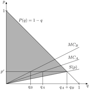
Example 1. Let P(q) = 1−p,CA(qA) = 16q2A andCB(qB) = 14q2B.
The social welfare for this example is depicted in Figure 1 by the shaded area when firms produce quantities qA= 1/2 and qB= 1/3.
q p
P(q) = 1−q
S(p) M CB
M CA
pc
qA+qB
qA
qB
1
1
Figure 1: Social welfare in the mixed Cournot duopoly.
In equilibrium firms produce quantities, which satisfy the equation system derived from the first-order conditions:
∂πAC(qA,qB)
∂qA =P0(qA+qB)qA+P(qA+qB)−CA0 (qA) = 0,
∂πBC(qA,qB)
∂qB =P(qA+qB)−CB0 (qB) = 0.
(3) From Tomaru and Kiyono (2010) it follows that under Assumptions 1 and 2 the equation system (3) has a unique solution and that the mixed Cournot duopoly has a unique equi- librium in pure strategies. In particular, we impose the concavity of the demand function by Assumption 1, which implies their Assumption 3. A minor difference in the imposed assumptions is that Tomaru and Kiyono (2010) assume demand curves not intersecting the horizontal axis in contrast to condition (i) of Assumption 1. However, this does not change
the fact that the firms’ reaction functions are differentiable, strictly decreasing and posses derivatives larger than−1 whenever they are positive. In our setting both reaction curves cut the respective axis at the horizontal intercept of the demand curve. Therefore, taking also point (ii) of Assumption 2 into account, the two firms’ reaction curves have a unique interception point.4
Coming back to Example 1, it can be verified that the Nash equilibrium of the mixed Cournot duopoly game is given byqA= 1/5 and qB = 8/15, while the equilibrium of the standard Cournot duopoly is given byqA= 9/29andqB= 8/29. Clearly, the mixed version of the Cournot duopoly results in larger outputs and social welfare.
2.2 The price-setting game
In this section we briefly review the result obtained by Balogh and Tasnádi (2012) on the simultaneous-move mixed Bertrand-Edgeworth duopoly with capacity constraints in which firms can produce up to their capacity levelskA, kB ∈(0, a]at zero unit costs after setting their prices simultaneously.5 Taking capacities as given, firms choose their pricespi∈[0, b]
(i=A, B) to maximize their payoffs.
To determine the firms’ demand and profit functions, we employ the efficient rationing rule.6 Let us denote the market clearing price by pc and firmi’s (i=A, B) unique profit- maximizing price on its residual demand curveDri(pi) = max{0, D(pi)−kj} bypmi in case ofkj < a, whereDri equals the demand faced by firmi if it is the high-price firm (j6=i).7 Letπir(pi) =piDir(pi). Any price leads to zero profits onπirin case ofkj =a, and therefore, for notational convenience we definepmi by 0in this case. Hence,
pc=P(kA+kB) and pmi = min
arg max
p∈[0,b]πir(p)
.
Furthermore, letpdi be the lowest price satisfying equation pdi min{ki, D(pdi)}=πri(pmi ),
whenever this equation has a solution.8 Thus, by choosing pdi and sellingmin{ki, D(pdi)},
4See also Amir and De Feo (2014, Section 5).
5The main assumption is that firms have identical unit costs when production takes place. For the case of asymmetric unit costs in the price-setting stage we refer to Deneckere and Kovenock (1996).
6Suppose firmicharges the lowest price (pi). Ifki< D(pi), not all consumers who want to buy from firmiare able to do so. The efficient rationing rule suggests that the most eager consumers are the ones who are able to purchase from firmi, that is the residual demand function of firm j6=ican be obtained by shifting the market demand function to the left byki. This rationing rule is called efficient because it maximizes consumer surplus. For more details we refer to Vives (1999) or Wolfstetter (1999).
7Deneckere and Kovenock (1992) define a similar price topmi ; however, in a slightly different way since they include firmi’s capacity constraint in the profit-maximization problem with respect toDri.
8The equation definingpdi has a solution if and only ifpmi ≥pc, which will be the case in our analysis when we will refer topdi.
firmigenerates the same amount of profit as it would by settingpmi and serving its residual demand.
Now we are coming back to definitions of the firms’ demand and profit functions. The firm which sets the lower price faces the market demand, while the firm with the higher price has a residual demand ofDir(pi) = max{0, D(pi)−kj}. In the case ofpA=pBthe following tie-breaking rule is used for mixed duopolies: If prices are higher than a thresholdp, which equals eitherpdA if pmA ≥pc or 0 otherwise, then the demand is allocated in proportion of the firms’ capacities, however if prices are not higher than p, the public firm allows the private firm to serve the entire demand up to its capacity level in order to encourage the private firm to set lower prices.9 Formally,
∆i(pi, pj) =
min{ki, D(pi)} if pi < pj, min{ki, Dir(pi)} if pi > pj, min{ki,kki
i+kjD(pi)} if pi =pj > p,
min{ki, D(pi)} if pi =pj ≤pand i=A, min{ki, Dir(pi)} if pi =pj ≤pand i=B.
(4)
The firms’ objective functions are given by
πAB(pA, pB) =pA∆A(pA, pB) (5) and
πBB(pA, pB) =
Z min{kj,max{0,D(pj)−ki}}
0
Rj(q)dq+
Z min{ki,a}
0
P(q)dq, (6)
where0≤pi ≤pj ≤b and Rj(q) = (Drj)−1(q).
For Example 1, we illustrate firms’ profits and consumers’ surplus in Figure 2. The lightest-grey triangle corresponds to the surplus realized by the consumers who purchase the product at the highest price, while the light-grey area depicts the surplus realized by the other consumers. On the producers’ side, the low-price firm’s surplus is given by the darkest-grey rectangular and the high-price firm’s surplus by the dark-grey area. Note that total welfare is determined by the higher price, except when the residual demand equals zero at the higher price.
The solution of the price-setting game can be found in Balogh and Tasnádi (2012, Propositions 2 and 5). IfpmA ≥pc, the equilibrium prices(p∗A, p∗B)are given by
p∗A=p∗B=pdA (7)
9For prices higher thanpwe could have used many other tie-breaking rules, e.g. the tie-breaking rule used by Kreps and Scheinkman (1983), the only requirement is that none of the firms should have the possibility to sell its entire capacity. For more about the employed tie-breaking rule we refer to Balogh and Tasnádi (2012).
q p
P(q) = 1−q Rj(q) = 1−q−ki
ki kA+kB pc
pi pj
Figure 2: Total welfare in the price-setting game or
n
(p∗A, p∗B)∈[0, b]2 |p∗A=pmA and p∗B≤pdAo
. (8)
Moreover, ifkB ≤kAandkB≤D(pM), wherepM is the price set by a monopolist without capacity constraints, i.e. pM = arg maxp∈[0,P(0)]pD(p), then price profiles
(p∗A, p∗B)∈[0, b]2 |p∗A= max{pM, P(kA)} and p∗B >max{pM, P(kA)} (9) are also equilibrium profiles.
If, howeverpmA < pc, then the set of equilibrium profiles equals
(p∗A, p∗B)∈[0, b]2 |p∗A=pc and p∗B≤pc . (10) Henceforward, we will refer to the first case (pmA ≥pc) as thestrong private firm case and to the latter (pmA < pc) as the weak private firm case.
In the strong private firm case the equilibrium given by (7) Pareto dominates the one given by (8). Furthermore, the not always existing equilibria given by (9) describe situations when the public firm is inactive, which would imply that the public firm does not care about consumer surplus and its own profits. Therefore in what follows we consider (7) as the solution of the price-setting game in the strong private firm case.10
Hence, firms’ equilibrium quantities are be given by
qA∗ = min{kA, D(p∗A)} and qB∗ = min{kB, DrB(p∗B)}. (11)
10For more details on selecting (7) as the most plausible equilibrium we refer to Balogh and Tasnádi (2012).
3 The mixed Kreps and Scheinkman game
In this section we determine the subgame perfect Nash equilibrium of the following two- stage game:
1. firms’ choose their capacity levels kA, kB ∈ [0, a] simultaneously at respective costs CA(kA), CB(kB) and
2. firms play the mixed price-setting game discussed in Subsection 2.2.
We will refer to this capacity then price game as the mixed Kreps and Scheinkman game.
Theorem 1. Under Assumptions 1, 2 and efficient rationing
• the mixed Cournot duopoly has a unique equilibrium (qA∗, qB∗),
• in a subgame perfect equilibrium, assuming that in case of a strong private firm in the second stage (7) is played, the mixed Kreps and Scheinkman game has a unique first-stage equilibrium (kA∗, kB∗) and
• (qA∗, qB∗) = (kA∗, kB∗).
Proof. We divide our proof into five steps.
Step 1. We identify and describe the capacity regions in which the first-stage profit functions are defined by different expressions.
The equilibrium prices of the subgame given by (7) or (10) are functions of the first- stage capacity decisions. Based on Berge’s Maximum Theorem the maximum residual profit πrA(pmA) is continuous in (kA, kB) and since pmA is unique it is a continuous function of(kA, kB) as well.11 Therefore,pdA is continuous in (kA, kB) on subregion
(kA, kB)∈[0, a]2 |pmA(kB)≥P(kA+kB) , i.e wheneverpdA is well defined.12
Let us denote the set of capacity-profiles compatible with the weak private firm case by Kc=
(kA, kB)∈[0, a]2|pmA(kB)≤P(kA+kB) and with the strong private firm case by
Kd=
(kA, kB)∈[0, a]2 |pmA(kB)> P(kA+kB) . Notice thatKc is a closed set, since pmA and P are continuous.
11In fact,pmA is independent fromkA, and therefore, in what follows we considerpmA as a single variable function.
12Note that, ifpmA =pc, thenpdA=pc.
We need to consider pmA, which by definition is the price maximizing p(D(p)−kB).13 That is,pmA satisfies the following first-order condition:
∂πrA
∂p (pmA) =pmAD0(pmA) +D(pmA)−kB= 0. (12) Based on Assumption 1, ∂π∂prA is strictly decreasing,pmA is unique and, as already mentioned, independent fromkA.
The boundary curve dividing the strong and the weak private firm case is given by pmA(kB) = P(kA+kB). For any given kB, if kA satisfiespmA(kB) = P(kA+kB), then for every capacitykA0 ∈[0, kA) we have that pmA(kB)< P(k0A+kB), which is the case because the left-hand side is independent ofk0A and the right-hand side is decreasing in kA0 . Thus, for every kB there exists ak00A such that the projection ofKcat kB equals[0, k00A].
We show that the boundary curve, which is defined by the implicit equation pmA(kB) = P(kA+kB), is strictly decreasing in (kA, kB) space. The implicit equation defining the boundary curve can be expressed as
D0(P(kA+kB))P(kA+kB) +kA+kB−kB= 0
from which under Assumption 1 by the Implicit Function Theorem we obtain
∂kB
∂kA = −D00(P(kA+kB))P0(kA+kB)P(kA+kB) +D0(P(kA+kB))P0(kA+kB) + 1 D00(P(kA+kB))P0(kA+kB)P(kA+kB) +D0(P(kA+kB))P0(kA+kB)
= −1− 1
P0(kA+kB) (D00(P(kA+kB))P(kA+kB) +D0(P(kA+kB))) <0.
Furthermore, let us divide Kdinto subsets K1d = n
(kA, kB)∈Kd|kA≤D
pdA(kA, kB)o and K2d =
n
(kA, kB)∈Kd|kA> D
pdA(kA, kB) o
,
wherepdA has been defined in Subsection 2.2 for given capacity profiles lying inKd. Hence- forth, we omit the arguments kA and kB of functions pdA, pmA and pc for notational conve- nience.
We turn to determining the projection of the setK1dat an arbitrarily fixed value ofkB. The condition kA ≤ D(pdA) defining K1d is equivalent to P(kA) ≥pdA, where by definition pdA= (pmA(D(pmA)−kB))/kA within K1d. We thus define:
f(kA) = pmA(D(pmA)−kB)
kA −P(kA) = c
kA −P(kA),
13Bear in mind that we have definedpmA separately for the case ofkB = a, ensuring that pmA is left- continuous ata.
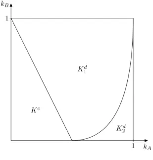
wherec=πAr(pmA)depends only onkB.14 While the sign off0is ambiguous,f00>0, that isf is strictly convex. Moreover,limkA→0+f(kA) =∞andf(a)>0. Let us denote the capacity level on the boundary of setsKcandKdatkB byk0A, that ispmA(kB) =P(kA0 +kB). It can be shown that f(k0A) < 0, thus for any given kB there exists a kA00 so that the projection of the set K1d equals (k0A, k00A]. Based on these results for any given kB the private firms capacities can be partitioned into three regions[0, k0A]× {kB} ⊂Kc,(k0A, k00A]× {kB} ⊂K1d and (k00A, a]× {kB} ⊂ K2d. Figure 3 illustrates the spatial arrangement of Kc, K1d and K2d for Example 1.
kA kB
Kd
1
Kd
2
Kc 1
1
Figure 3: Set of capacities
Step 2. We show that the first-stage equilibrium capacities cannot lie inK2d. IfkA≤D(pdA), then
pdAkA=pmA(D(pmA)−kB) ⇐⇒ pdA= pmA(D(pmA)−kB)
kA , (13)
while forkA> D(pdA),pdA is defined by the minimum price satisfying equality
pdAD(pdA) =pmA(D(pmA)−kB). (14) Note, however, that this latter case cannot be part of the equilibria, sincepdA given by (14) is independent of kA, and for that reason the private firm could increase its profit by choosing a lower capacity level equal to kA0 = kA−ε > D(pdA). Thus, in equilibrium kA≤D(pdA) holds.
14Observe that in the strong private firm caseπrA(pmA)>0andD(pmA)−kB>0.
Step 3. We show that the first-stage equilibrium capacities cannot lie inK1d.
Given the equilibrium prices, for any capacity profile (kA, kB) the firms’ first-stage objective functions are
πA(kA, kB) =
pdAkA−CA(kA) if (kA, kB)∈Kd,
pckA−CA(kA) if (kA, kB)∈Kc (15) and
πB(kA, kB) =
( RD(pdA)
0 P(q)dq−CA(kA)−CB(kB) if (kA, kB)∈Kd, RkA+kB
0 P(q)dq−CA(kA)−CB(kB) if (kA, kB)∈Kc. (16) For simplicity we did not substitute the already determined expressions for functions pdA andpcin the objective functions.
Since solutions from Kc and K1d dominate the capacity levels from K2d we focus our attention only onKc and K1d. However, by determining ∂k∂
AπA(kA, kB) on the interior of K1d we can exclude capacities belonging to K1d as well. To see this, consider the private firm’s profit function on the above mentioned interval:
πA(kA, kB) =pdAkA−CA(kA) =pmA(D(pmA)−kB)−CA(kA),
thus ∂
∂kA
πA(kA, kB) =−C0(kA)<0.
Hence, πA is decreasing in kA on K1d for any givenkB, which implies that the equilibrium solution is necessarily inKc.
Step 4. We show that the unique equilibrium (q∗A, qB∗) of the mixed Cournot duopoly lies in Kc and satisfies the first-order condition of the first-stage of the mixed Kreps and Scheinkman game.
Notice that within Kc the objective functions given by (15) and (16) are identical to (1) and (2) determined for the mixed Cournot duopoly case. We express the second period residual profit function definingpmA in terms of quantities and maximize
πAr(qA) =P(qA+kB)qA
with respect to qA, where kB =q∗B, and letkA=q∗A. The solution is denoted asqmA. For this problem the sufficient first-order condition yields
P0(qmA +kB)qAm+P(qAm+kB) = 0. (17) Observe that P(qAm +kB) coincides with pmA(kB), since we have solved the same profit maximization problem in two different ways. Combining equation (17) and the first equation of (3), we get
P0(qAm+kB)qmA +P(qmA +kB)−CA0 (kA)< P0(kA+kB)kA+P(kA+kB)−CA0 (kA) = 0
by Assumption 2. Therefore, since functionP0(qA+kB)qA+P(qA+kB)is strictly decreasing inqA on [0, a−kB]by Assumption 1 it follows that qAm > kA, which in turn implies that pmA(kB) =P(qAm+kB)< P(kA+kB). Thus, (qA∗, qB∗) lies in the interior ofKc.
Step 5. We show that the unique equilibrium of the mixed Cournot duopoly is indeed an equilibrium of the first-stage of the mixed Kreps and Scheinkman game.
As explained in Subsection 2.1 the first-order conditions given by (3) have a unique solution, now denoted by(kA∗, kB∗), and thus the capacity-choice game can have at most one equilibrium in pure strategies with(k∗A, kB∗)as the potential equilibrium solution. We check that(k∗A, k∗B)is an equilibrium of the capacity-choice stage, which means that for both firms we have to exclude a unilateral and beneficial deviation in capacity falling into regionKd. Concerning the private firm, we have already seen that πA(k∗A, kB∗) > πA(kA, k∗B) for any (kA, k∗B) ∈ Kd. Turning to the public firm, by increasing its capacity from kB∗ until the boundary of Kc decreases social welfare, and increasing kB even further results in lower social welfare than in case of the mixed Cournot duopoly sincepdA(k∗A, kB)> P(kA∗, kB) for any(kA∗, kB)∈Kd.
Informally, Theorem 1 means that quantity precommitment and Bertrand competition yield Cournot outcomes not only in duopolies with private firms (see Kreps and Scheinkman, 1983) but also in mixed duopolies.
References
Amir, R. and De Feo, G. (2014): Endogenous Timing in a Mixed Duopoly, International Journal of Game Theory, Vol. 43, No. 3, 629–658.
Bakó, B. and Tasnádi, A. (2014): A Kreps-Scheinkman állítás érvényessége lineáris keresletű vegyes duopóliumok esetén? (The Kreps and Scheinkman Result Remains Valid for Mixed Duopolies with Linear Demand),Közgazdasági Szemle, Vol. 61, No 5, 533–543 (in Hungarian).
Balogh, T.L. and Tasnádi, A. (2012): Does Timing of Decisions in a Mixed Duopoly Mat- ter?,Journal of Economics, Vol. 106, No. 3, 233–249.
Beato, P. and Mas-Colell, A. (1984): The Marginal Cost Pricing as a Regulation Mechanism in Mixed Markets, in Marchand, M., Pestieau, P. and Tulkens, H. eds.,The Performance of Public Enterprises, North-Holland, Amsterdam, 81–100.
Boccard, N. and Wauthy, X. (2000): Bertrand Competition and Cournot Outcomes: Fur- ther Results,Economics Letters, Vol. 68, No. 3, 279–285.
Boccard, N. and Wauthy, X. (2004): Bertrand Competition and Cournot Outcomes: A Correction,Economics Letters, Vol. 84, No. 2, 163–166.
Cremer, H., Marchand, M. and Thisse, J.-F. (1989): The Public Firm as an Instrument for Regulating an Oligopolistic Market, Oxford Economic Papers, Vol. 41, No. 2, 283–301.
Davidson, C. and Deneckere, R. (1986): Long-Run Competition in Capacity, Short-Run Competition in Price, and the Cournot Model,Rand Journal of Economics, Vol. 17, No.
3, 404–415.
Deneckere, R. and Kovenock, D. (1992): Price Leadership, Review of Economic Studies, Vol. 59, No. 1, 143–162.
Deneckere, R. and Kovenock, D. (1996): Bertrand-Edgeworth Duopoly with Unit Cost Asymmetry,Economic Theory, Vol. 41, No. 1, 1–25.
de Fraja, G. and Delbono, F. (1989): Alternative Strategies of a Public Enterprise in Oligopoly,Oxford Economic Papers, Vol. 41, No. 2, 302–311.
de Frutos, M.-A. and Fabra, N. (2011): The Role of Demand Uncertainty, International Journal of Industrial Organization, Vol. 29, No. 4, 399–411.
George, K. and La Manna, M.M.A. (1996): Mixed Duopoly, Inefficiency, and Public Own- ership,Review of Industrial Organization, Vol. 11, No. 6, 853–860.
Harris, R.G. and Wiens, E.G. (1980): Government Enterprise: An Instrument for the Internal Regulation of Industry, Canadian Journal of Economics, Vol. 13, No. 1, 125–
132.
Kreps, D.M. and Scheinkman, J.A. (1983): Quantity Precommitment and Bertrand Compe- tition Yiels Cournot Outcomes,The Bell Journal of Economics, Vol. 14, No. 2, 326–337.
Lepore, J.J. (2009): Consumer Rationing and the Cournot Outcome, The B.E. Journal of Theoretical Economics, Vol. 9, No. 1 (Topics), Article 28.
Lepore, J.J. (2012): Cournot Outcomes under Bertrand-Edgeworth Competition with De- mand Uncertainty, Journal of Mathematical Economics, Vol. 48, No. 3, 177–186.
Loertscher, S. (2008): Market Making Oligopolies, Journal of Industrial Economics, Vol.
56, No. 2, 263–289.
Merrill, W.C. and Schneider, N. (1966): Government Firms in Oligopoly Industries: A Short-run Analysis, Quarterly Journal of Economics, Vol. 80, No. 3, 400–412.
Osborne, M.J. and Pitchik, C. (1986): Price Competition in a Capacity-Constrained Duopoly,Journal of Economic Theory, Vol. 38, No. 2, 238–260.
Reynolds, S.S. and Wilson, B.J. (2000): Bertrand-Edgeworth Competition, Demand Uncer- tainty, and Asymmetric Outcomes,Journal of Economic Theory, Vol. 92, No. 1, 122–141.
Tomaru, Y. and Kiyono, K. (2010): Endogenous Timing in Mixed Duopoly with Increasing Marginal Costs, Journal of Institutional and Theoretical Economics, Vol. 166, No. 4, 591–613.
Vives, X. (1999): Oligopoly Pricing: Old Ideas and New Tools, MIT Press, Cambridge MA.
Wolfstetter, E. (1999): Topics in Microeconomics, Cambridge University Press, Cambridge UK.
Wu, Xin-wang, Zhu, Quan-tao and Sun, Laixiang (2012): On Equivalence Between Cournot Competition and the Kreps–Scheinkman Game, International Journal of Industrial Or- ganization, Vol. 30, No. 1, 116–125.