Evaluating neural network and linear regression photovoltaic power forecasting models based on different input methods

(1)

Contents lists available atScienceDirect

Energy Reports

journal homepage:www.elsevier.com/locate/egyr

Research Paper

Evaluating neural network and linear regression photovoltaic power forecasting models based on different input methods

Mutaz AlShafeey

^∗

, Csaba Csáki

Department of Information Systems, Institute of Informatics, Corvinus University of Budapest, Budapest, Fővám tér 13-15, H-1093, Hungary

a r t i c l e i n f o

Article history:

Received 17 March 2021

Received in revised form 12 September 2021 Accepted 31 October 2021

Available online xxxx Keywords:

Solar energy

Photovoltaic technology Prediction model Multiple regression Artificial neural network Prediction accuracy

a b s t r a c t

As Photovoltaic (PV) energy is impacted by various weather variables such as solar radiation and temperature, one of the key challenges facing solar energy forecasting is choosing the right inputs to achieve the most accurate prediction. Weather datasets, past power data sets, or both sets can be utilized to build different forecasting models. However, operators of grid-connected PV farms do not always have full sets of data available to them especially over an extended period of time as required by key techniques such as multiple regression (MR) or artificial neural network (ANN). Therefore, the research reported here considered these two main approaches of building prediction models and compared their performance when utilizing structural, time-series, and hybrid methods for data input.

Three years of PV power generation data (of an actual farm) as well as historical weather data (of the same location) with several key variables were collected and utilized to build and test six prediction models. Models were built and designed to forecast the PV power for a 24-hour ahead horizon with 15 min resolutions. Results of comparative performance analysis show that different models have different prediction accuracy depending on the input method used to build the model: ANN models perform better than the MR regardless of the input method used. The hybrid input method results in better prediction accuracy for both MR and ANN techniques, while using the time-series method results in the least accurate forecasting models. Furthermore, sensitivity analysis shows that poor data quality does impact forecasting accuracy negatively especially for the structural approach.

1. Introduction

Irrespective of all the advantages of utilizing photovoltaic (PV) technology for energy production, there are some hindrances lim- iting growth and wider utilization. One of the crucial drawbacks of solar solutions is low energy converting efficiency (Huang et al., 2013). Other drawbacks come from the nature of solar radiation which, unfortunately, highly fluctuates over time leading to generation uncertainty. Fluctuation and uncertainty in energy production lead to uncertainty in economic benefits.

Calculating economic indicators such as energy pricing, rate of return, and payback period is challenging under generation uncertainty. Additionally, uncertainty can affect grid stability in case of grid-connected PV farms (Alshafeey and Csáki,2019).

There are many solutions that have been used to overcome the above problems, but most of them are either costly (such as batteries Koohi-Fayegh and Rosen,2020) or maybe impractical in several situations (e.g. hybrid diesel generators Yamegueu et al.,2011; Cavalcante et al.,2021). One promising solution is

∗ Correspondence to: Budapest, Fővám tér 13-15, H-1093, Hungary.

E-mail addresses: Mutaz.AlShafeey@uni-corvinus.hu(M. AlShafeey), Csaki.Csaba@uni-corvinus.hu(C. Csáki).

to enhance solar energy forecasting (Singh,2013;Devaraj et al., 2021). If potential solar energy can be accurately predicted with lower uncertainty, solar systems can be better designed and optimized helping grid operators in managing power supply and demand (Pazikadin et al., 2020). Accurate forecasts would improve grid stability as well (Rodríguez et al., 2018). Improving the forecasting models is one of the most important aspects of solar energy production and is considered to be one of the

‘hottest’ topics in the solar energy research field. Solar energy prediction models are software solutions that can be used to forecast future values of solar power generation. The forecasting horizon is the time between the present and the effective time of the predictions, while forecasting resolution is the frequency of the predictions (Antonanzas et al., 2016). Like any system that predicts the future, the forecasted value of energy would have a degree of uncertainty and errors. A good prediction model can forecast future values with minimum errors and uncertainties (Cammarano et al.,2012).

A potential problem with such forecasting models concerns the ability of grid-connected PV farm operators to utilize their advantages. Operators may not be familiar with the different techniques and hiring relevant expertise might be costly, but more importantly, they often face a situation when they do not have

https://doi.org/10.1016/j.egyr.2021.10.125

(2)

all necessary data available to train such models successfully.

Therefore, the main aim of the research reported here was to clarify the effects of utilizing different input data configurations on the forecasting accuracy in order to help PV grid-connected farms to achieve better forecasting accuracy within the available data that is normally collected from PV farms. Different PV farms have different data depending on the sensors installed or their budget (to purchase data from 3rd party). The study presented here aimed to evaluate different methods for building PV solar power forecasting models each utilizing different combinations of real PV solar power, geographical, and meteorological variables as input. As a result, three methods of utilizing input data – structural, time-series and hybrid – were used to build statistical (multiple regression - MR) and machine learning (ANN) prediction models. The datasets used for building and testing the models were collected from a 546 kWp grid-connected solar farm. The performance of the six models utilizing different configurations of the available input data were then evaluated.

Hence grid operators can consider the best model based on the data available to them. This manuscript expands on prior research conducted and published in the field, yet the novelty of this work is derived from three aspects. First, prior researches either focus on one modelling technique utilizing different input data methods or focus on different modelling techniques utilizing one input data method — however, this work focuses on both. Second, the design and test of the models are the results of a systematic approach followed by a comprehensive performance analysis over several measures. And finally, the dataset is an outcome of the operation of a grid-connected PV farm, thus the testing results are not simulated, instead, they are outcomes based on large amount of real-life data under various weather conditions over several years.

The paper is organized as follows. After the introduction, PV solar energy forecasting methods are reviewed. This is followed by an overview of the methodology applied where the source data and model approaches used are described. The main section deals with the evaluation of various methods, models, and their settings — resulting in some potential improvement options. The paper closes with conclusions and future research.

2. PV solar energy forecasting methods

Solar power forecasting is a sophisticated process, many factors affect its accuracy. Other than the choice or combination of modelling methods, selecting forecast horizon and forecast model inputs (prediction variable patterns) are key decisions to be made (Ahmed et al.,2020). In addition, there are several measures established to show performance and compare accuracy of solutions (these would include various forms of error calculations among others and are discussed in detail in Section3.3.3).

The forecasting horizon is the time between the present and the effective time of the predictions (Antonanzas et al., 2016).

Although thus far there is no international classification crite- rion (Nespoli et al.,2019;Sobri et al.,2018), most studies cate- gorize forecasting horizon into three classes: short-term (up to 48–72 h ahead), medium-term (from a few days to one week ahead), and long-term forecasting (from a few weeks to a year or more ahead) (Mellit et al., 2020; Raza and Khosravi, 2015;

de Marcos et al.,2019). The second factor that affects the prediction model accuracy is the set of input variables. Choosing the right variables is one of the challenges in designing PV power forecasting models (Ahmed et al., 2020). Selecting input variables imprudently increases cost, computational complexity, and forecasting errors (Raza et al.,2016).

One of the simplest techniques to forecast solar energy is using the average values of historical solar energy and weather

records (Abunima et al., 2019). However, the average method is not suitable because averages do not represent the full range of values, which will be reflected by having some considerable errors in the forecasted values. Furthermore, those errors and the inherent uncertainty of solar radiation will be aggravated, leading to additional uncertainty (Linguet et al.,2016).

Two competing key techniques for solar power forecasting are statistical calculations and machine learning (Das et al., 2018).

Machine Learning (ML) is the study of computer algorithms that are able to improve automatically through ‘experience’. ML models can solve complex problems by establishing complex rela- tions between inputs and outputs and their performance usually depends on the quality and quantity of data available for training (Harrington,2012). They have been used for many purposes including classification, pattern recognition, spam detection, and they are also used in data mining and forecasting problems (Voy- ant et al., 2017). Machine learning techniques are divided into supervised, unsupervised, and meta-learning algorithms (Lantz, 2019). Each of these algorithms has one or more learning tasks, i.e. supervised learning algorithms can be used for numeric prediction and classification problems, while unsupervised learning algorithms can be used for pattern detection and cluster- ing (Lantz, 2019). One of the supervised learning algorithms is Artificial Neural Networks (ANN). The ANN technique can solve complex nonlinear, nonanalytical, and nonstationary stochastic problems without complex programming required (Inman et al., 2013).

The above abilities and advantages have influenced many re- searchers to use ANN in solar forecasting — including irradiation and energy production prediction (Wang et al.,2019a). As a result, a rising number of research reports and ANN-based forecasting applications have been published in the past 20 years (Garud et al.,2021). For example, ANN is used to forecast day-ahead solar energy with 1-hour forecasting resolutions utilizing historical weather data as well as time-series power data (Chen et al., 2011). ANN has also been applied as a base for short-term solar power prediction models (Almonacid et al.,2014) that showed a good performance for 1-hour power forecasting. Three different short-term prediction models using ANN were built inOudjana et al.(2013). The first model utilized temperature data to forecast power and showed huge errors; the second model utilized solar irradiance data which resulted in better forecasting accuracy;

while the third model showed the best accuracy and it utilized both temperature and solar irradiance to forecast power. ANN PV power forecasting model based on a self-organizing feature map (SOFM) was proposed inYousif et al.(2017), where the suggested model uses solar irradiance and ambient temperature to forecast PV power. The results show that using ANN based on SOFM im- proves prediction accuracy. Real-time solar irradiance was used to make two-hour-ahead solar irradiance levels forecasting in Vanderstar et al.(2018): the proposed method uses ANN to forecast the irradiance and genetic algorithm to optimize array size and position in order to obtain the most accurate prediction. The suggested method shows adequate forecasting capabilities, yet, it has some limitations as this method only works for non-zero solar Global Horizontal Irradiance (GHI) values. InNotton et al.(2019) ANN models were proposed to forecast different solar irradiance components for 1 to 6-hour horizons. The results show that ANN is a very promising method to forecast solar radiation. Several ANN forecasting models were proposed to predict hourly solar irradiance in six different locations in Nigeria (Bamisile et al., 2020). The results show that all of the proposed ANN models performed well and can be used for PV performance calculation.

Multiple weather variables such as temperature, precipitation, wind speed, and solar irradiation were used to build a multi- channel convolutional neural network (CNN) prediction model in

7602

(3)

Table 1

Forecasting methods, horizons, resolutions, and variables.

Reference Forecast horizon Forecast resolution Methods Variables

Oudjana et al.(2012) 7 days 24 h Linear regression, MR, neural network Global irradiance, temperature Al-Messabi et al.(2012) 10 and 60 min. 10 and 60 min Dynamic ANN Actual and past values of power

Ogliari et al.(2013) 24 hours- 1 h ANN hybrid approach Weather variables

De Giorgi et al.(2014) 1–24 h 1–24 h Statistical methods based on MR analysis; ANN

PV power, module temperature, ambient temperature, solar irradiance

Chu et al.(2015) 5–15 min. 5 min. Many methods including cloud tracking, k-NN, ANN

Power past values and sky images

Leva et al.(2017) 24 hours- 1 h ANN Power and solar radiation past values,

Numerical Weather Prediction variables Pitalúa-Díaz et al.(2019) 30 days 5 min MR, Gradient Descent Optimization

(GDO) and Adaptive Neuro-Fuzzy Inference System (ANFIS)

Solar radiation, ambient temperature, wind speed, daylight hour and PV power

Heo et al. (2021). The suggested model extracts meteorological as well as geographical features of PV sites from raster image datasets. The results show high forecasting capabilities, however, to avoid any biased prediction, sufficient data should be included.

ANN was the most applied technique for solar power forecasting over the last ten years especially for short-term prediction as 48% of related articles published between 2009–2019 were using ANN (Mellit et al.,2020).

Unlike ML methods which formulate solar energy prediction problems as a black box, statistical methods reveal the math- ematical relationship between the input variables and the output (Wang et al., 2020a). Such statistical methods include Au- toregressive Moving Average (ARMA), Auto-Regressive Integrated Moving Average (ARIMA), exponential smoothing, and regression (Wang et al.,2020b; Das et al.,2018). Multiple Linear Re- gression (MLR) is also popular in PV solar power forecasting (e.g. De Giorgi et al., 2014; Oudjana et al., 2012; Pitalúa-Díaz et al.,2019). Regression methods establish a relationship between the explanatory (meteorological and geographical) variables and dependent variables (the forecasted PV power) (Das et al.,2018).

Table 1 provides a brief chronological overview of the main PV forecasting methods applied for different horizons using various resolutions and input variables.

To forecast solar power, prediction models may utilize different parameters as inputs. Choosing among potential variables depends on the availability of related data for the required location and time period (as some locations do not have full datasets covering all the required parameters and for an extended period of time). Depending on the parameters used – i.e. the so-called explanatory variables utilized – the prediction models can be built using three different approaches (Aggarwal and Saini,2014;

Bacher et al.,2009;Jafarzadeh et al.,2012;Khatib et al.,2012):

• structural methods that only utilize the geographical and meteorological parameters as inputs;

• time-series methods that only utilize the historical data of solar power as inputs; and

• hybrid methods that utilize solar power historical data as well as other variables like geographical and meteorological parameters as inputs.

It should be noted, that there are two basic approaches to time-series forecasting: direct forecasting and multi-step rolling forecasting. While in the direct approach only actual historical data is utilized (i.e. always being one-time horizon behind), in the rolling approach the predictions of the previous values are used like they were actual values when predicting the next value (being one resolution step behind). Although there are some claims that multi-step rolling forecasting is slightly better than the direct option for certain tasks (see for example Lan et al.,

2019for frequency-based solar irradiation forecasting), for solar power output this method has been found to be problematic. This is because the error generated in each step is propagated to the subsequent steps (Sahoo et al.,2020). Thus, it is found to be less accurate due to the accumulation of the error along the prediction horizon (Galicia et al.,2019). Consequently, this paper focuses on direct time-series forecasting.

While ANN and MLR are heavily studied methods, most of the literature focus either on testing one method of modelling utilizing different variables (see for exampleInman et al.,2013;

Oudjana et al., 2013) or on testing different methods utilizing the same variables (such asOgliari et al.,2013;Chu et al.,2015;

De Giorgi et al.,2014), the goal of this study was to compare and analyse the performance of two different modelling techniques – namely ANN and multiple regression – for PV power forecasting each using all three above-mentioned methods of utilizing input data. For instance, ANN solar radiation forecasting model was proposed and benchmarked with MLR and ARIMA models using satellite-derived land-surface temperature (LST) as an input predictor for 21 stations in Queensland (Deo and Şahin,2017). Even though the study uses satellite-derived data to enhance solar radiation forecasting accuracy, yet the authors suggested future studies to test for shorter time-scale, as well as utilizing satellite data merged with reanalysis and ground-based products. Another study evaluated the PV power forecasting performance of different ANN models and some simple statistical models like ARMA, ARIMA, and Seasonal Auto-Regressive Integrated Moving Average (SARIMA) (Sharadga et al., 2020), yet, only time series of the power output was utilized. In study (Qu et al.,2021) time-series data of PV power and some related weather variables namely radiation, temperature, and humidity were utilized in different combinations to build a hybrid neural network forecasting model (composed of attention-based, long-term, and short-term tempo- ral parts, i.e. ALSM). The proposed model shows better forecasting accuracy than ARMA and ARIMA models. However, only one input data method was utilized (hybrid time-series input data). Hence, compared with existing research on similar topics this paper provides a comprehensive comparison of PV solar power forecasting options and systematically evaluates the effectiveness and appli- cability of deterministic predictors over two different methods.

Moreover, the main goal of this research was to assist operators of PV grid-connected farms to achieve better forecasting accuracy depending on the data available to them in an industrial situation.

Solar farm operators do not necessarily have full sets of data that includes (all) geographical and meteorological parameters as well as past power, especially over an extended period of time.

Therefore, it is essential for them to be able to judge the expected accuracy they may achieve depending on the data available and to make smart decision which method (or methods) to use.

(4)

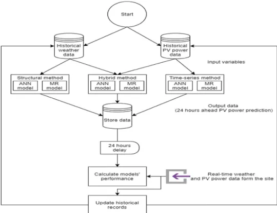
Fig. 1. General overview of the methodology flowchart.

Source:Authors.

3. Design of the experiment and methods 3.1. Objective and research methodology

Key challenges facing solar energy forecasting models include the task of choosing the right method and the need to select appropriate inputs to achieve the most accurate prediction. Con- sequently, the research reported here aimed at investigating two of the main techniques for building prediction models to accurately forecast PV output production: multiple regression (MR) and artificial neural network (ANN). To that end, structural, time- series, and hybrid data input methods were used to build different forecasting models and experiment with different input (predictor) settings.

Fig. 1 depicts a general overview of the steps forming the development process. Building the forecasting models starts by feeding the historical weather and PV power data to the models.

Structural models are fed with historical weather data, time- series models are fed with historical PV power data, while hybrid models are fed with both weather and PV power historical data.

Each model is forecasting the PV output power for the selected horizon with a given resolution set (for details see next Subsec- tion). The forecasted PV output power values are then stored.

When the real values become available as a fact data from the PV farm, this data is used to calculate the performance of each model (i.e. in comparison to the stored prediction) as well as to update the historical data records (which means this real-time data is later applied to update the model).

As part of the research, a large amount of historical data was collected to build the prediction models. The data collected covered the period April 13, 2017 to April 18, 2020 (3 years). The data used to train the models for prediction is measured data. Past data is used as an input to forecast the next day, albeit differently depending on input method. For example the measurement of April 13 had been used to predict expected output for April 14

in case of the structural model, and for April 15th in cases of the time-series and hybrid models. In other words, for the structural model weather data from exactly 24 h earlier is used to forecast for a given point in time – e.g. any timeslot of April 14 may be predicted using data from April 13. However, for the time series data prediction (and, therefore, for the hybrid model as well) a full past day data of generated power is needed as input for the model to forecast the next day – e.g. a prediction done on April 14 to predict the same timeslot on April 15 (one-day- ahead) uses data covering a full 24 h going back (thus including data from April 13), consequently, no prediction is possible for April 14 if data is not available from April 12. This was repeated until April 18, 2020. Thus, all models were continuously trained and tested over the data covering a 3-year period. For all ANN models trained here, the data was split into three segments: 70%

training 15% validation, and 15% test set. Since this implies tens of thousands of values of each variable, it would be hard to visualize the forecasted versus the real power values for the whole period.

Therefore, the last day of testing (18th of April 2020) was used to visualize and compare the performance of the different models.

This day appeared to be a good test day as it had a few dips during the day due to weather changes during the day (as opposed to an average stochastic PV power curve).

3.2. Data and data collection

To achieve the aims of this study, large amount of data is required to build and test the proposed prediction models. Thus, various sources were used to collect data. Two international firms were collaborating with the authors to provide the necessary historical and real-time data. A Hungarian operator of several large farms provided the authors with full access to the power generation data of a grid-connected PV farm using SolarEdge farm man- agement interface. While geographical and meteorological data for the solar farm location were provided by a specialized firm of- fering solar data services, Solcast Technologies.Table 2shows the

7604

(5)

Table 2

Technical site information.

Location Hungary

Date of the establishment April 13th, 2017

Peak power kWp 546

Data obtained Energy and power generated (every 15 min)

PV cell model ND-RJ260

Number of modules 2100

Number of inverters 18

PV solar farm site specifications including location, peak power, established date, data obtained, and other technical information.

Cell temperature was not provided by the data source, hence it was calculated using Eq.(1)(Mattei et al.,2006;Trinuruk et al., 2009):

T_c=T_a+(^Ts−20)∗solar irradiance

800 (1)

whereT_c,^Ta, andT_sare the cell, ambient, and the Standard Test Conditions (STC) temperature in Celsius. TheTsfor the PV models used for this study is 25^◦.

Historical weather data records include air temperature, cloud opacity, dewpoint temperature, Diffuse Horizontal Irradiance (DHI), Direct Normal Irradiance (DNI), Direct Beam Horizontal Irradiance (EBH), Global Horizontal Irradiance (GHI), Global Tilted Irradiance (GTI) fixed-tilt, GTI Tracking, precipitable water, relative humidity, snow depth, and wind speed. These variables are described in Table 3(all collected with 15 min resolutions between April 13, 2017, and April 18, 2020).

3.3. Major factors affecting solar power forecast

This section presents the forecast horizons, forecast model inputs, and performance estimation measures used in this study.

3.3.1. Forecast horizon

Forecasting horizon is one of the major factors that affect forecasting accuracy (Das et al.,2018). The relationship between the forecasting horizon and accuracy is reverse: forecasting accuracy decreases significantly for longer horizons (Ahmed et al.,2020).

As this research was designed to help grid-connected PV farms to achieve better forecasts within the available data, the models are intended to forecast 24 h ahead as the day-ahead PV energy forecasting is of the utmost importance in decision-making pro- cesses (Cococcioni et al.,2011). Moreover, certain grid operators in the European Union (EU) are required to report a 24-hours- ahead with 15 min resolution forecast from each grid-connected PV farm (Orasch,2009;Zsiborács et al.,2019).

3.3.2. Forecast model inputs

PV power output is highly correlated with weather variables (Wang et al., 2019b). Yet, not all weather variables have the

Table 4

The correlation between PV output power and meteorological variables.

Input variables Correlation with PV output power

Air temperature 0.42

Cloud opacity −0.26

Dewpoint temperature 0.18

DHI 0.68

DNI 0.84

EBH 0.87

GHI 0.95

GTI fixed tilt 0.96

GTI tracking 0.90

Precipitable water 0.09

Relative humidity −0.53

Snow depth −0.09

Wind speed 10 m 0.09

Cell temperature 0.52

same significance for PV power forecasting. A correlation analysis was done to determine the significance of each collected variable shown inTable 3before it was used in the modelling: seeTable 4 for results.

As can be seen inTable 4, some meteorological factors have higher significance than others. Solar irradiance components have the highest significant factors, especially GTI fixed-tilt. Generally, it can be concluded that all variables collected here can be used in the modelling, yet variables that have low correlations with the output power could be excluded: in this study the threshold is set to 0.1, therefore wind speed, snow depth, and precipitable water are excluded.

3.3.3. Performance calculations

Subsequently, a comparative performance analysis between the resulting models shall be executed in order to compare prediction results and identify the most accurate model depending on specified evaluation criteria. To evaluate the performance of the forecasting model, one or more evaluation methods are needed. Accuracy of the forecasting models can be evaluated using Mean Absolute Error (MAE), Mean Squared Error (MSE), Coefficient of Determination (COD), Error (ε), and Root Mean Square Error (RMSE).Table 5summarizes those methods (Ahmed et al., 2020; Elsheikh et al., 2019), where n is the number of observations,y_tandp_t are the observed (real) and the forecasted output power values at timet, respectively, andyˆis the average of the observed values.

MAE is a quantity that is used in order to measure the close- ness of the predicted values to the measured values. MSE measures the average of the squares of the errors – and thus embodies not only how widely the estimates are spread from the real sample but also how far off the average estimated value is from the true value. COD has been used to show how close prediction model results are to the actual measured data line as a fitted regression line (also known as R-squared (R²) score and is generally used for testing hypotheses). Error is the actual (not

Table 3

Variables used in the study.

Name Type Unit Source

Air temperature Historical weather Celsius Solcast

Cell temperature Calculated Celsius Calculations

Wind speed Historical weather m/s Solcast

Cloud opacity Historical weather Percentage (%) Solcast

Dewpoint temperature Historical weather Celsius Solcast

DHI, EBH, DNI, GHI, and GTI Historical weather W/m² Solcast

Precipitable water Historical weather Centimetres Solcast

Relative humidity Historical weather Percentage (%) Solcast

Snow depth Historical weather Centimetres Solcast

PV power generation Historical power W SolarEdge

Forecasted PV power Predicted variable W Prediction model output

(6)

absolute) value of the difference between the estimation and the corresponding actual value. RMSE is calculated to measure the prediction of a given approach thus shows the so-called scattering level produced by the model. For higher modelling accuracy, MAE, MSE, εand RMSE indices should be closer to zero but the COD value should be closer to 1.

4. The PV power forecasting models used

Both forecasting techniques, multiple regression and ANN were applied to the dataset (as prepared in Section 3.2) using three different methods: structural, time-series, and hybrid — leading to six models in total. Regression models were developed using R packages, while ANN models were built in Matlab.

4.1. Multiple regression model and its three variants

A multiple linear regression model for PV power forecast can be denoted as follows:

y=β0+β1v1+β2v2+β3v3+β4v4+ · · · +βnvn+ε ⁽²⁾ wherev1,v2, . . . ,vnare the input variables (1 to n). The coefficient β0 is the intercept, while values ofβ1, . . . ,βn denote the slope coefficient of each input (explanatory) variable, andεis the error (the amount by which the predicted value is different from the actual value). The regression model estimates the best values of β1, . . . ,βnleading to least errorε^.

Given all or part of the explanatory variables (Table 3), the multiple regression model can be used to forecast PV output power (y) for a given timet. To forecast future values ofywithin the forecast horizon (i.e. y_(t+₁₎,^y(t+₂₎, . . . ,^y(t+_h), whereh is the number of time periods between the present and the effective time of predictions), past values of v are required. Since the resolution is 15 min, to forecast one day ahead h is set to 96 time periods. Consequently, for a given time t, y is predicted usingvvalues from time (t−h). Notice, that as explained under methodology, forecasting should start on the second day of data collection to avoid negative times.

In structural method, the input variables fed to the multiple regression model are only the meteorological and geographical variables — with low correlation variables left out according to Section3.3.2. Past values of selected weather variables were utilized according to Eq.(3)which denotes the Structural Multiple Regression model (SMR):

y₍_t₎=β0+β1v1(t−_h)+β2v2(t−_h)+β3v3(t−_h)+ · · · +βnvn(t−_h)+ε ⁽³⁾ PV output power can be forecasted by knowing its past values (Cococcioni et al.,2011). Therefore, for the time-series method only PV output power values were used as input such that actual past PV output power values were used to predict future values (y(t)) of the output power according to Eq.(4)which denotes the Time-series Multiple Regression model (TMR):

y(^t)= ˆβ0+ ˆβ1y_(t−h−0)+ ˆβ2y_(t−h−1)+ · · · + ˆβhy_(t−h−95)+ε ⁽⁴⁾ where βˆ1, . . . ,βˆh denote the slope coefficient of each input (explanatory) variable, exactly as explained earlier, the hat symbol used here just to indicate that each model has its unique beta values.y_(t−_h−₀₎,^y(t−_h−₁₎, . . . ,^y(t−_h−₉₅₎are the past PV power values starting from 24 h before the forecasting takes place (i.e. 24 h before the 1st prediction) and goes until 48 h before the 1st prediction. In other words, y_(t−_h−₀₎ is the past PV power value 24 h (96 time period) before forecastingy₍_t₎,y_(t−_h−₁₎represents the past PV power value 97 time period before forecasting y₍_t₎, andy_(t−_h−₉₅₎represents the past PV power value 191 time period before forecasting y₍_t₎. So, for predictingy₍_t₎, 96 past PV power values are utilized by the model. Note that to forecast y₍_t₎, the

Table 5

Definitions of performance measures.

Measure Equation

Mean Absolute Error (MAE) MAE=¹

n∗

n

∑

i=1

|yt−pt|

Mean Squared Error (MSE) MSE=¹

n∗

n

∑

i=1

(^yt−pt)² Coefficient of Determination (COD) R²=

∑n

i=1(^y^t−pt)²

∑n i=1

(yt− ˆy)₂

Error ε=yt−pt

Root Mean Square Error (RMSE) RMSE=





√ 1 n∗

n

∑

i=1

(^yt−pt)²

past PV power values 48 h prior to the forecast are required, thus the first day of forecasting PV output power by TMR model was April 15th, 2020. This ensures that there is no overlap between the prediction horizon period (of 24 h) and the data representing the actual power generated, which becomes available at the end of each day.

Finally, in the hybrid method past values of all the variables, including actual past values of the power variable as well as past values of the weather variables were fed to the model to predict future PV output power values as shown in Eq.(5)representing the Hybrid Multiple Regression model (HMR):

y(^t)=β0+β1v1(t−_h)+β2v2(t−_h)+β3v3(t−_h)

+ · · · +βnvn(t−h)+ ˆβ1y_(t−h−0)+ ˆβ2y_(t−h−1)

+ · · · + ˆβhy_(t−_h−₉₅₎+ε ⁽⁵⁾ whereβ0is the intercept for the HMR model.

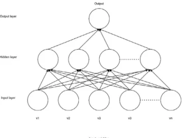
4.2. Artificial neural network (ANN) model and its three variants ANN is a network of ‘‘neurons’’ that are arranged in a layered structure. Fig. 2 shows a simple diagram of ANN where input variables arrive from the bottom, while the forecasted variable(s) (output) appears at the top layer. An ANN also includes one or more hidden layers and hidden neurons. Such an ANN structure where the information flow is directed in one direction only (from the bottom to the top layer) is called Multi-Layer Feed-Forward Neural Network (MLFFNN). Note that in this work MLFFNN networks are used. In order to evaluate the performance of the training algorithm performance, the error (difference between the MLFFNN output and the real measured output) is determined using MSE equation in Table 5. To minimize MSE values between the observed real output and the forecasted output back-propagation algorithm is used where MSE values are utilized to update the weights and the biases of the network.

In MLFFNN, each layer receives its inputs from the previous layer (except for the input layer), so the outputs of a certain layer are the inputs to the next one. Inputs to each neuron in a given (hidden or output) layer are combined using a weighted linear combination. Then a nonlinear activation (transfer) function ϕ modifies the results before it is ready to be output. This network structure has many advantages for this forecasting context as this structure works well with big data and provides quick predictions after training. Moreover, it can be applied to solve complex non-linear problems and same accuracy ratio can be achieved even with even smaller data (Khishe et al., 2018; Akkaya and Çolakoğlu,2019).Fig. 3shows the flow of information in one artificial neuron, wherew1,w2,. . . ,wnare the weights corresponding to input datav1,v2, . . . ,vnrespectively (Kim,2017).

7606

(7)

Fig. 2. A neural network with n inputs and one output.

Source:Authors.

Fig. 3. Flow of information in an artificial neuron.

Source:Authors.

Before reaching the neuron, the input signal of each neuron from the previous layer is multiplied by its dedicated weight.

Once the weighted signals are collected, they are added to create the weighted sum (ws) as denoted by Eq.(6), wherebis the bias for the neuron:

ws=w1×v1+w2×v2+ · · · +wn×vn+b (6) The weighted sum equation can be written with matrices as in(7)(Kim,2017):

ws=wv+b (7)

wherew^andvare defined as:

w= [w1w2w3 . . . wn]andv=

⎡

⎢

⎣ v1

v2

v3

.. v.n

⎤

⎥

⎦

(8)

Then finally, the neuron enters the weighted sum into the activation function and yields its output as shown in Eq.(9):

X=ϕ⁽ws) (9)

One of the most used activation functions is the sigmoid function (Ghritlahre and Prasad,2018) as given by(10):

ϕ (ws)= ¹

1+e⁻^w^s (10)

Note that the sigmoid function is replaced by the Tansig transfer function whenever negative values are found in the input or output layers (Ghritlahre and Prasad,2018) as follows:

ϕ (ws)= ¹−e⁻²^w^s

1+e⁻²^w^s (11)

The above equations represent one neuron but each individual neuron has its own specific set of weights and bias on the inputs.

The weights of neurons are initially set to random values. Training data is fed to the bottom (input) layer and it passes through the succeeding layers, getting multiplied and added together as described in the equations, until it finally arrives, drastically transformed, at the output layer. Information is stored in form of weights. Those weights have to be changed to train the ANN with new information. In this work back-propagation algorithm is applied to minimize the MSE between the real observed output and forecasted output from the MLFFNN, the weights are adjusted in proportion to the input value(s) and the output error (MSE) as can be seen in(12)(Talaat et al.,2020).

Min (MSE)=min(1 n∗

n

∑

i=₁

(^yt−p_t)²⁾ ⁽¹²⁾

The change in weights and biased are calculated as in(13)and (14)respectively (Talaat et al.,2020;Leema et al.,2016):

∆wn=γ^(yn−p_n) (13)

∆^bn=γ^(yn−p_n) (14) where∆wnis the change of weight for thenth neuron,∆^bnis the change of the bias for thenth neuron, andγ is the learning rate.

Subsequently, the adjusted weights (wadjusted) and biases (b_adjusted) are donated as in(15)and(16)respectively.

wadjusted=w+_∆w ⁽¹⁵⁾

b_adjusted=b+_∆b (16)

One unit of this process (when training data is passed forward through the neural network and then the weights of each neuron are adjusted based on the error) is called an epoch. During training, the weights are repeatedly adjusted each epoch. This loop will continue until either a specific number of epochs is reached or when the value of MSE reaches the lowest possible limit (typically when MSE does not change for several epochs).

This research utilizes a fully connected MLFFNN as described above with one hidden layer. For each of the three methods used, the ANN was fed with the same set of input variables as were the corresponding MR models. Notice, this implies a differing number of input neurons for each method used. The number of input neurons, therefore, are 11, 96, and 107 for the structural, time series, and hybrid input methods respectively. The number of hidden neurons is an important parameter for ANN. With few hidden neurons the ANN might not be able to generate a function that indicates the underlying problem while having more hidden neurons than required may result in over-fitting of the training set and reducing the ability of generalization the out-of-sample data (Setyawati,2005). Therefore the number of hidden neurons was set to be 33% (one-third) of the number of inputs.Table 6 shows the settings of the ANN parameters. Although training time had not been limited, the actual running time for the set number of epochs to be trained was ranging from seconds to a couple of hours, while forecasting times were, of course, very short (fraction of a second).

(8)

Table 6 ANN parameters.

Parameter Description Value for each method

Structural Time series Hybrid

Number of inputs Number of input data variables 11 96 107

Number of outputs Number of output forecasted variables 1 1 1

Number of hidden neurons Number of hidden neurons 4 32 35

Maximum epochs Maximum number of training iterations before training is stopped 1000 1000 1000

Maximum training time Maximum time in seconds before training is stopped Unlimited Unlimited Unlimited

Performance goal The minimum target value of MSE 0 0 0

Fig. 4. Frequency distribution of the error in SMR.

Source:Authors.

5. Results of the experiments and discussion

After developing the suggested models, a series of experiments were constructed to measure the performance of each model variant and to compare their prediction abilities using the evaluation measures described inTable 5. The overall (average) performance of each variant was computed at the end of training and testing (i.e. over 3 years). Then, as an additional demonstration that enables some representative visualization, the performance for forecasting the output power for 18th of April 2020 was also computed and compared to the overall performance (seeTable 7).

5.1. Multiple regression models

Initially, the multiple regression model was developed utilizing only meteorological and geographical variables, then another MR model was built to utilize only time-series data of PV solar power, and finally, a third model was developed utilizing both PV power historical data as well as geographical and meteorological parameters as inputs (for details see Section4.1).

5.1.1. Structural Multiple Regression model (SMR) performance Over the training and testing period, this model shows a good performance with a 0.94 COD, 14.84 MAE, 1054.74 MSE, and, 32.47 RMSE.Fig. 4shows the frequency distribution of the error.

It can be seen that the most frequent errors recorded are small errors ranging between−20 and+20 kW. However, some fairly large errors can also be observed.

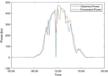
The SMR model was able to forecast the energy for the 18th of April with a 0.92 COD, 22.44 MAE, 1815.52 MSE, and, 42.60 RMSE performance measures. Which is a bit less than the overall performance.Fig. 5shows the forecasted vs. observed power for the mentioned day.

Note that the model utilizes real values, that is they have 100%

accuracy. This explains the very good prediction performance.

In case meteorological parameters can only be provided with some degree of uncertainty, the SMR might have less accurate

Table 7

Performance measures comparison.

Model Performance measures

COD (R²) MAE MSE RMSE

MR SMR 0.94 14.84 1054.74 32.47

TMR 0.68 45.83 5584.5 74.72

HMR 0.95 16.05 835.68 28.90

Average 0.86 25.57 2491.64 45.36

ANN SANN 0.95 13.13 943.53 30.26

TANN 0.75 36.38 4329.87 36.38

HANN 0.96 13.52 914.10 30.23

Average 0.89 21.01 2062.5 32.29

Fig. 5. Forecasted vs. observed power for the SMR.

Source:Authors.

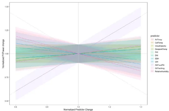
performance. Fig. 6 shows a sensitivity analysis for the SMR model where the effect of uncertainty in the input variables can be observed on the forecasted power.

The sensitivity analysis shows the normalized percent changes in the forecasted PV output power with the normalized percent of input variables uncertainty. The point (1,1) on the graph represent 100% accurate inputs, therefore, there is no change in forecasted power. An uncertainty between 0 and±40% in any of the input variables (i.e. 0.6 and 1.4 in the x-axis) leads to huge changes in the model’s output, thus affecting the performance.

5.1.2. Time-series Multiple regression model (TMR) performance Over the training and testing period, this model shows poor performance, much worse than the SMR with a 0.68 COD, 45.83 MAE, 5584.5 MSE, and, 74.72 RMSE.Fig. 7shows the frequency distribution of the error. Some huge errors were recorded, additionally, the errors are not distributed around zero (most frequent errors do not equal zero)

Fig. 8shows the forecasted vs. observed power for the 18th of April 2020. It can be noticed from error measures andFig. 8 that the TMR performs worse than the SMR. The TMR could not

7608

(9)

Fig. 6. Sensitivity analysis for the SMR model.

Source:Authors.

Fig. 7. Frequency distribution of the error in TMR.

Source:Authors.

predict the sudden drop in the output PV power just before noon, while this drop was better predicted by the SMR.

The SMR model was able to forecast the energy for the 18th of April with a 0.88 COD, 32.97 MAE, 3091.27 MSE, and, 55.59 RMSE performance measures. Which is above the overall performance of this model. This can be explained as the 18th of April does not have huge weather variations, thus the TMR performs better than other days.

5.1.3. Hybrid Multiple regression model (HMR) performance Over the training and testing period, this HMR model shows the best overall performance compared to TMR and SMR, with a 0.95 COD, 16.05 MAE, 835.68 MSE, and, 28.90 RMSE.Fig. 9shows the frequency distribution of the error. Even though the HMR shows better performance, yet it shows more errors between−50 and 50 kW.

The HMR model was able to forecast the energy for the 18th of April with 0.93 COD, 22.26 MAE, 1796.84 MSE, and, 42.38

Fig. 8. Forecasted vs. observed power for the TMR.

Source:Authors.

RMSE performance measures. Which is a bit less than the overall performance.Fig. 10shows the forecasted vs. observed power for that day.

5.2. Artificial neural network models

The ANN models were built the same way as were the MR models in Section 5.1. Initially, the ANN model was developed utilizing only selected meteorological and geographical variables, then another ANN model was developed to utilize only time- series data of PV power, and finally, a third ANN model was developed to utilize PV power historical data as well as geographical and meteorological parameters as inputs.

5.2.1. Structural Artificial Neural Network model (SANN) perfor- mance

Over the training and testing period, this model shows a good performance with a 0.95 COD, 13.13 MAE, 943.53 MSE, and, 30.26 RMSE. The SANN reached the best performance (least MSE) after

(10)

Fig. 9. Frequency distribution of the error in HMR.

Source:Authors.

Fig. 10. Forecasted vs. observed power for the HMR.

Source:Authors.

140 epochs as shown inFig. 11. The error distribution is inFig. 12 which shows the total frequency of errors as well as the error frequency in the training, validation, and test sets.

The TMR model was able to forecast the energy for the 18th of April with 0.93 COD, 20.96 MAE, 1752.54 MSE, and, 41.86 RMSE performance measures. Which is a bit less than the overall performance.Fig. 13shows the forecasted vs. observed power for that day.

5.2.2. Time-series Artificial Neural Network model (TANN) perfor- mance

Over the training and testing period, this model shows a fair performance, slightly better than the TMR with a 0.75 COD, 36.38 MAE, 4329.87 MSE, and, 36.38 RMSE. The TANN reached the best performance (least MSE) after 241 epochs (Fig. 14). The error distribution can be found inFig. 15.

The TANN model was able to forecast the energy for the 18th of April with 0.87 COD, 32.57 MAE, 3135.32 MSE, and, 55.99 RMSE performance measures. Which is better than the overall performance but no dip is predicted, for the same reason mentioned in5.1.2.Fig. 16shows the forecasted vs. observed power for the mentioned day.

Fig. 11. SANN performance.

Source:Authors.

Fig. 12. Frequency distribution of the error in SANN.

Source:Authors.

Fig. 13. Forecasted vs. observed power for the SANN.

Source:Authors.

5.2.3. Hybrid Artificial Neural Network model (HANN) performance Over the training and testing period, the model shows a good performance, way better than the TANN with a 0.96 COD, 13.52 MAE, 914.10 MSE, and, 30.23 RMSE. The HANN reached the best performance (least MSE) after 29 epochs as shown inFig. 17. The error distribution can be found inFig. 18.

7610

(11)

Fig. 14. TANN performance.

Source:Authors.

Fig. 15. Frequency distribution of the error in TANN.

Source:Authors.

Fig. 16. Forecasted vs. observed power for the TANN.

Source:Authors.

Fig. 17. HANN performance.

Source:Authors.

Fig. 18. Frequency distribution of the error in HANN.

Source:Authors.

The HANN model was able to forecast the energy for the 18th of April with 0.94 COD, 19.0 MAE, 1626.35 MSE, and, 40.32 RMSE performance measures. Which is almost the same as the expected performance.Fig. 19shows the forecasted vs. observed power for the mentioned day with the daily dip predicted.

5.3. Performance comparison

In this section, a performance comparison for all the models that were designed and tested in the previous subsections is provided.Table 7summarizes the overall performance data of the different models.

AsTable 7shows, the difference between MR and ANN is very clear in the time-series data, where TANN performance is highly superior compared to TMR. Moreover, even though SMR and SANN show comparable performances, yet the SMR is sensitive to the uncertainty in the input variables as discussed in the sensitivity analysis of Section5.1.1. HANN has the highest COD, and the lowest MSE, and RMSE, thus the HANN has the best overall performance in all the measures used except MAE where SANN has the lowest value. It can be noticed that ANN is generally overperformed MR models — as can also be observed from the

(12)

Fig. 19. Forecasted vs. observed power for the HANN.

Source:Authors.

diagrams inFig. 20which show average overall performance for the MR and ANN.

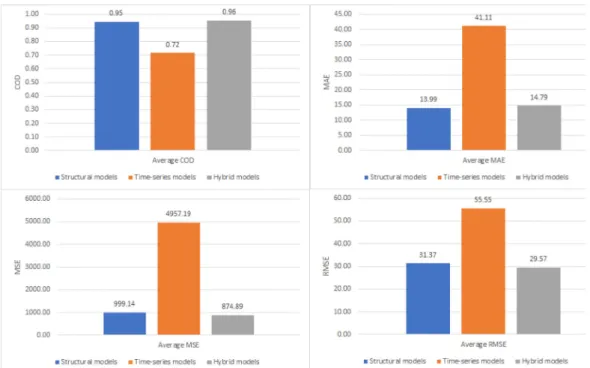
Fig. 21shows average performance measures comparison between structural, time-series, and hybrid methods. Time-series models have the worst performances. Although hybrid and structural models have close performance values, hybrid models perform vaguely better in the MSE and RMSE measures, while structural models overperform the hybrid ones in the MAE measure.

When comparing the performance of the models for forecasting PV output power on April 18th, 2020 similar conclusions can be made, as expected: ANN models were slightly overperforming MR ones (seeTable 8).

Here again, time-series models show unfavourable performance compared to the structural or hybrid models. The hybrid models show the highest COD and least MAE, MSE, and RMSE.

6. Conclusions

This paper demonstrates two different techniques of PV energy prediction modelling, namely ANN and MR. Depending on

the input variables utilized, forecasting models were built using three different approaches: structural, time-series, and hybrid.

The six models were built to predict the PV solar power for a 546 kWp grid-connected solar farm located in Hungary. This research is targeted to help PV farms improving their power prediction, therefore, the horizon and the resolution of the forecasts were set based on the forecasting regulations affecting certain grid operators in the European Union. Hence, all forecasting models were built and designed to forecast PV output power for a 24-hour ahead horizon with 15 min resolution. So, a historical data set including 3-years of geographical and meteorological variables was collected for the site of this specific PV farm along with actual PV power values. This data was used to build, train, and test the models.

The results indicate that ANN forecasting models have higher COD and lower MAE, MSE, RMSE values compared to the MR, regardless of the method used for building the forecasting models.

It was also found that using the hybrid method to build prediction models results in better prediction accuracy for both MR and ANN while using the time-series method results in the least accurate forecasting models.

After analysing the results of this work using real farm data, it was confirmed that ANN technique performs better than the MR. This is true regardless of the input method used to build the models. It was also found that using the hybrid method of input data to build the forecasting models leads to better forecasting accuracy regardless of the technique used. The results of sensitivity analysis show that input variables and corresponding data quality have huge effects on the models’ output when utilizing the structural technique. Consequently, in case of poor data quality or inaccurate weather data it is recommended to avoid using the structural method, especially when using the structural method to build MR forecasting models. To summarize, farm operators may have better results using ANN-based models with hybrid input approach.

Finally, some improvements might be done to expand this work. One possibility is to compare the performance of the tested forecasting models for different horizons and resolutions. In the- ory, the performance of the forecasting models is decreasing for longer forecasting horizons. It would be worthwhile to study the performance of the tested models for medium- and long-term forecasting horizons.

Fig. 20. Average performance measures comparison between MR and ANN.

Source:Authors.

7612

(13)

Fig. 21. Average performance measures comparison between structural, time-series, and hybrid models.

Source:Authors.

Table 8

Performance measures comparison for PV out power for the 18th of April 2020.

Model Performance measures

COD (R²) MAE MSE RMSE

MR SMR 0.92 22.44 1815.52 42.60

TMR 0.88 32.97 3091.27 55.59

HMR 0.93 22.26 1796.84 42.38

Average 0.91 25.89 2234.54 46.86

ANN SANN 0.93 20.96 1752.54 41.86

TANN 0.87 32.57 3135.32 55.99

HANN 0.94 19.0 1626.35 40.32

Average 0.91 24.18 2171.40 46.06

CRediT authorship contribution statement

Mutaz AlShafeey:Conceptualization, Methodology, Software, Formal analysis, Investigation, Writing – original draft. Csaba Csáki: Validation, Writing - original draft, Writing – review &

editing, Methodology, Supervision.

Declaration of competing interest

The authors declare that they have no known competing finan- cial interests or personal relationships that could have appeared to influence the work reported in this paper.

Acknowledgements

Our Artificial Application for Renewable Energy Production Prediction project is supported by solar irradiance and weather data from Solcast (http://solcast.com). Solar power plant operation data is provided by 3Comm Hungary (3comm.hu/). Project no. TKP2020-NKA-02 has been implemented with the support provided by the National Research, Development and Innovation Fund of Hungary, financed under the ‘Tématerületi Kiválósági Program’ funding scheme.

References

Abunima, H., Teh, J., Jabir, H.J., 2019. A new solar radiation model for a power system reliability study. IEEE Access 7, 64758–64766.

Aggarwal, S., Saini, L., 2014. Solar energy prediction using linear and non-linear regularization models: A study on AMS (American Meteorological Society) 2013–14 Solar Energy Prediction Contest. Energy 78, 247–256.

Ahmed, R., Sreeram, V., Mishra, Y., Arif, M., 2020. A review and evaluation of the state-of-the-art in PV solar power forecasting: Techniques and optimization.

Renew. Sustain. Energy Rev. 124, 109792.

Akkaya, B., Çolakoğlu, N., 2019. Comparison of Multi-class Classification Algo- rithms on Early Diagnosis of Heart Diseases. y-BIS Conference 2019: Recent Advances in Data Science and Business Analytics, İstanbul, Turkey, p. 162–72.

Al-Messabi, N., Li, Y., El-Amin, I., Goh, C., 2012. Forecasting of photovoltaic power yield using dynamic neural networks. In: The 2012 International Joint Conference on Neural Networks (IJCNN). IEEE, pp. 1–5.

Almonacid, F., Pérez-Higueras, P., Fernández, E.F., Hontoria, L., 2014. A methodology based on dynamic artificial neural network for short-term forecasting of the power output of a PV generator. Energy Convers. Manage. 85, 389–398.

Alshafeey, M., Csáki, C., 2019. A case study of grid-connected solar farm control using artificial intelligence genetic algorithm to accommodate peak demand.

J. Phys. Conf. Ser. 012017, IOP Publishing.

Antonanzas, J., Osorio, N., Escobar, R., Urraca, R., Martinez-de Pison, F.J., Antonanzas-Torres, F., 2016. Review of photovoltaic power forecasting. Sol.

Energy 136, 78–111.

Bacher, P., Madsen, H., Nielsen, H.A., 2009. Online short-term solar power forecasting. Sol. Energy 83, 1772–1783.

Bamisile, O., Oluwasanmi, A., Obiora, S., Osei-Mensah, E., Asoronye, G., Huang, Q., 2020. Application of deep learning for solar irradiance and solar photovoltaic multi-parameter forecast. Energy Sour. Part A: Recovery, Util. Environ. Effects 1–21.

Cammarano, A., Petrioli, C., Spenza, D., 2012. Pro-energy: A novel energy prediction model for solar and wind energy-harvesting wireless sensor networks. In: 2012 IEEE 9th International Conference on Mobile Ad-Hoc and Sensor Systems (MASS 2012). IEEE, pp. 75–83.

Cavalcante, R.L., Costa, T.O., Almeida, M.P., Williamson, S., Galhardo, M.A.B., Macêdo, W.N., 2021. Photovoltaic penetration in isolated thermoelectric power plants in Brazil: Power regulation and specific consumption aspects.

Int. J. Electr. Power Energy Syst. 129, 106648.

Chen, C., Duan, S., Cai, T., Liu, B., 2011. Online 24-h solar power forecasting based on weather type classification using artificial neural network. Sol. Energy 85, 2856–2870.

Chu, Y., Urquhart, B., Gohari, S.M., Pedro, H.T., Kleissl, J., Coimbra, C.F., 2015.

Short-term reforecasting of power output from a 48 MWe solar PV plant.

Sol. Energy 112, 68–77.