Probabilistic Models in Weather Forecasting

(1)

Probabilistic Models in Weather Forecasting

Dissertation submitted for the degree of

“Doctor of the Hungarian Academy of Sciences”

S´ andor Baran

Debrecen, 2019

(2)

(3)

Acknowledgements

Here I would like to thank all the people who have, either directly or indirectly, contributed to this dissertation.

First of all to my wife, ´Agnes for her love, patience, understanding and standing always by me.

To my daughters Zsuzsanna and J´ulia for bringing so much joy into my life.

To my parents for helping and encouraging me.

To Tilmann Gneiting, who motivated my research in probabilistic forecasting and su- pervised my first steps in this area, hosted me several times in Heidelberg, and gave an enormous help with his comments, remarks and suggestions.

To Andr´as Hor´anyi for introducing me atmospheric science, his help and collaboration.

To Sebastian Lerch for the fruitful collaboration, great ideas and all his help with the R codes.

To Annette M¨oller for her help with copula models and for collaboration.

To Stephan Hemri for introducing me hydrological forecasting and helping with the analog-based approaches.

To Martin Leutbecher and Zied Ben Bouall`egue for the collaboration and for hosting me several times at the European Centre for Medium-Range Weather Forecasts.

To all current and former members of the Computational Statistics Group of the Hei- delberg Institute for Theoretical Studies for providing an inspiring working environment.

Besides my collaborators special thanks to Kira Feldmann, Alexander Jordan, Fabian Kr¨uger and Roman Schefzik.

To my current and former students Mailiu D´ıaz Peña, Mehrez El Ayari, Dóra Nemoda and Marianna Szabó for their hard work in the field of probabilistic forecasting and tolerating me as their supervisor.

(4)

iv ACKNOWLEDGEMENTS Further, I would like to thank the following organizations and projects for providing the financial background of my research.

• DAAD programs “Research Stays for University Academics and Scientists, 2015”

and “Research Stays for University Academics and Scientists, 2017.”

• EFOP-3.6.1-16-2016-00022 project co-financed by the European Union and the Eu- ropean Social Fund.

• EFOP-3.6.3-VEKOP-16-2017-00002 project co-financed by the Hungarian Govern- ment and the European Social Fund.

• European Centre for Medium-Range Weather Forecasts.

• Hungarian Scientific Research Fund under Grant No. OTKA NK101680.

• J´anos Bolyai Research Scholarship of the Hungarian Academy of Sciences (2015–

2018).

• National Research, Development and Innovation Office under Grant No. NN125679.

• Visiting Scientist Program of the Heidelberg Institute for Theoretical Studies for years 2016 and 2018.

• T ´AMOP-4.2.2.C-11/1/KONV-2012-0001 project supported by the European Union and co-financed by the European Social Fund.

Finally, I am grateful

to the University of Washington MURI group for providing the University of Washington mesoscale ensemble data;

to Mih´aly Sz˝ucs from the Hungarian Meteorological Service for the ALADIN-HUNEPS data;

to the German Federal Office of Hydrology, and in particular Bastian Klein, for providing the hydrological data.

(5)

List of abbreviations

ALADIN-HUNEPS Aire Limitée Adaptation dynamique Développement International-Hungary Ensemble Prediction System ALARO Aire Limitée Application de la Recherche à l’Operationnel ARPEGE Action de Recherche Petite Echelle Grande Echelle

BfG German Federal Institute of Hydrology

BFGS Broyden-Fletcher-Goldfarb-Shanno (algorithm)

BMA Bayesian Model Averaging

BS Brier Score

BSS Brier Skill Score

CDF Cumulative Distribution Function COSMO Consortium for Small-Scale Modelling CRPS Continuous Ranked Probability Score CRPSS Continuous Ranked Probability Skill Score CSG Censored and Shifted Gamma (distribution)

DM Diebold-Mariano (test)

DS Determinant Sharpness

DST Daylight Saving Time

ECMWF European Centre for Medium-Range Weather Forecasts

EE Euclidean Error

EM Expectation-Maximization (algorithm) EMOS Ensemble Model Output Statistics

ENS (51-member ECMWF) Ensemble

EPS Ensemble Prediction System

ES Energy Score

GEFS Global Ensemble Forecast System

GEV Generalized Extreme Value (distribution)

GLAMEPS Grand Limited Area Model Ensemble Prediction System HIRLAM High Resolution Limited Area Modelling

HMS Hungarian Meteorological Service HRES (ECMWF) High-Resolution (forecast)

ISBA Int´eractions Soil Biosphere Atmosph`ere (parametrization scheme) LEPS Limited-Area Ensemble Prediction System

LN Log-Normal (distribution)

LogS Logarithmic Score

(6)

vi LIST OF ABBREVIATIONS MAE Mean Absolute Error

ML Maximum Likelihood

NCEP National Center for Environmental Prediction NWP Numerical Weather Prediction

PDF Probability Density Function PEARP Pr´evision d’Ensemble ARPEGE PIT Probability Integral Transform RMSE Root Mean Square Error

STRACO Soft Transition Condensation (parametrization scheme) SURFEX Surface Externalis´ee (parametrization scheme)

TN Truncated Normal (distribution)

twCRPS Threshold-Weighted Continuous Ranked Probability Score twCRPSS Threshold-Weighted Continuous Ranked Probability Skill Score UTC Coordinated Universal Time

UWME University of Washington Mesoscale Ensemble

(7)

Introduction

Capturing and modelling uncertainty is an essential need in any forecasting problem, and in weather or hydrological prediction it may result in an enormous economical benefit.

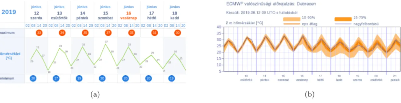
In the early 90’s there was an important shift in the practice of weather forecasting from deterministic forecasts obtained using numerical weather prediction (NWP) models in the direction of probabilistic forecasting. The crucial step was the introduction of ensemble prediction systems (EPSs) in operational use in 1992 both at the European Centre for Medium-Range Weather Forecasts (ECMWF) and the U.S. National Meteorological Cen- ter. An EPS provides a range of forecasts corresponding to different runs of the NWP models, which are usually generated from random perturbations in the initial conditions and the stochastic physics parametrization. In the last decades, the ensemble method has become a widely used technique all over the world as using ensemble forecasts one can, for instance, easily provide prediction intervals reflecting to forecasts uncertainty. The ad- vantage of ensemble forecasting is nicely illustrated by Figure 1 showing point forecasts of temperature for Debrecen, Hungary, and the corresponding ECMWF ensemble forecasts.

In the latter case (Figure 1b) the ensemble mean can serve as a point forecast, however, one can also observe how the forecast uncertainty increases with the increase of the lead time of prediction. Note that both forecasts are available for public on the official web page of the Hungarian Meteorological Service (www.met.hu).

However, raw ensemble forecasts often exhibit systematic errors as they might be biased or badly calibrated calling for some form of post-processing. Simple approaches to bias correction or calibration have a long history, however, in the first years of the XXI.

century several more sophisticated methods appeared (Wilks, 2006), including parametric models providing full predictive distributions of the weather variables at hand. Starting with the fundamental works of Tilmann Gneiting and Adrian Raftery (Gneiting and Raftery, 2005; Gneitinget al., 2005; Raftery et al., 2005) introducing Bayesian model averaging (BMA) and ensemble model output statistics (EMOS) for ensemble calibration, statistical post-processing of ensemble forecasts became a hot topic both in statistics and in atmospheric sciences, resulting in a multitude of probabilistic models for different weather quantities, new methods of estimation of parameters of these models and novel approaches to forecast verification (Buizza, 2018). Recently, the German Meteorological Service uses a special EMOS post-processing model (Schuhen et al., 2012) in operational wind vector prediction for the Frankfurt Airport, and there are ongoing research projects e.g. at the ECMWF pointing towards the introduction of statistical calibration in operational use (see e.g. Gneiting, 2014; Richardson et al., 2015; Baran et al., 2019b).

This dissertation is a summary of the achievements of the author in the area of probabilistic forecasting. It contains new BMA and EMOS models for post-processing of water levels and different weather quantities, novel approaches to training data selection in the

(10)

2 INTRODUCTION

(a) (b)

Figure 1: Point forecasts (a) and ECMWF ensemble forecasts (b) of temperature for Debrecen, Hungary. On panel (b) light and dark orange belts correspond to 80 % and 50 % central prediction intervals. Source: www.met.hu

parameter estimation process, and in some cases efficient algorithms for parameter estimation are also provided. Note that the presented results are purely applied. Due to the nature of the problems investigated, the verification of the proposed models and algorithms can be based only on carefully chosen case studies, which is a standard approach in probabilistic weather prediction. Using appropriate verification scores the forecast skill of each suggested method is compared with the predictive performance of the corresponding state of the art calibration models. The current work is mainly based on eight papers of the author published either in statistical journals (Computational Statistics and Data Analysis, Environmetrics, Journal of the Royal Statistical Society: Series C) or in journals in the field of atmospheric (Meteorology and Atmospheric Physics, Quarterly Journal of the Royal Statistical Society) or water sciences (Water Resources Research), but some results of other published journal articles are also used.

The dissertation consists of six main chapters. Chapter 1 introduces the basic notions of ensemble forecasting and statistical post-processing, lists the main parametric post- processing approaches and parameter estimation strategies and describes the methods of forecast evaluation. In Chapter 2 a novel BMA post-processing model for calibration of ensemble forecasts of water levels is proposed (Baran et al., 2019a) together with an efficient expectation-maximization (EM) algorithm based maximum likelihood (ML) method for parameter estimation. Chapter 3 deals with calibration of wind speed forecasts. It describes a new BMA approach (Baran, 2014) and two different EMOS models (Baran and Lerch, 2015, 2016) together with the existing up to date methods. In Chapter 4 a novel EMOS model for probabilistic quantitative precipitation forecasting (Baran and Nemoda, 2016) is compared with the existing parametric approaches. Joint calibration of wind speed and temperature ensemble forecasts is investigated in Chapter 5 by introducing bivariate BMA (Baran and Möller, 2015) and EMOS (Baran and Möller, 2017) models and comparing their predictive performance with the more general Gaussian copula approach (Möller et al., 2013). The fundamental part of the dissertation ends with Chapter 6, where two semi-local methods for choosing training data for post-processing models are described, followed by a short chapter containing some general conclusions.

Finally, we would like to mention that the implementation of the presented methods resulted in thousands of lines of R code (R Core Team, 2019) and most of the EMOS approaches considered in Chapters 3 and 4 are now available to a wide range of users as parts of the ensembleMOS package (Yuen et al., 2018) ofR.

(11)

Chapter 1 Probabilistic forecasts and forecast evaluation

1.1 Ensemble forecasts

The main objective of weather forecasting is to give a reliable prediction of future atmospheric states on the basis of observational data, prior forecasts valid for the initial time of the predictions, and mathematical models describing the dynamical and physical behaviour of the atmosphere. These models numerically solve the set of the hydro- thermodynamic non-linear partial differential equations of the atmosphere and its coupled systems. A disadvantage of these NWP models is that since the atmosphere has a chaotic character the solutions depend on the initial conditions and also on other uncertainties related to the numerical weather prediction process. In practice it means that the results of such models are never fully accurate and the forecast uncertainties should be also taken into account in the forecast preparation. One can reduce the uncertainties by running the model with different initial conditions resulting in an ensemble of forecasts (Leith, 1974). Using a forecast ensemble one can estimate the probability distribution of future weather variables which opens the door for probabilistic weather forecasting (Gneiting and Raftery, 2005), where not only the future atmospheric states are predicted, but also the related uncertainty information such as variance, probabilities of various events, etc.

Since its first operational implementation (Buizzaet al., 1993; Toth and Kalnay, 1997), this approach has became a routinely used technique all over the world and recently all major weather prediction centres have their own operational EPSs, e.g. the 30-member Consortium for Small-scale Modelling (COSMO-DE) EPS of the German Meteorological Service (Gebhardt et al., 2011; Ben Bouallègue et al., 2013), the 35-member Prévision d’Ensemble ARPEGE¹ (PEARP) EPS of Méteo France (Descamps et al., 2015) or the 51-member EPS of the independent intergovernmental ECMWF (ECMWF Directorate, 2012; Molteni et al., 1996; Leutbecher and Palmer, 2008), whereas the Hungarian Mete- orological Service (HMS) operates the 11-member Aire Limitée Adaptation dynamique Développement International-Hungary Ensemble Prediction System (ALADIN-HUNEPS;

Hor´anyi et al., 2006). It is also worth mentioning the experimental 8-member University of Washington mesoscale ensemble (UWME; Eckel and Mass, 2005), as an example of an EPS operated not by a weather centre.

1Action de Recherche Petite Echelle Grande Echelle (i.e. Research Project on Small and Large Scales)

(12)

4 CHAPTER 1. PROBABILISTIC FORECASTS AND FORECAST EVALUATION

2 4 6 8 10 12 14

24681012

Newport Municipal Airport, Oregon, USA

Day in October 2008

Wind speed (m/s)

− −

−

− − − − − −

− −

−

− − −

−

− − − − −

− −

−

− −

−

− − − − −

− − − −

−

− − − − − − −

− −

−

− −

−

− − − − − −

− −

−

− − −

−

− −

−

− − −

− −

−

− − −

−

− −

−

− −

−

− −

−

− −

−

− − −

−

2 4 6 8 10 12 14

0510152025

Debrecen Airport, Hungary

Day in December 2010

Precipitation accumulation (mm)

−

− − − −

−

− −

−

− −

−

− − − − − −

−

− − − − −

−

− − − − −

−

− −

−

− − −

−

− − − − − −

−

− − −

− −

− − − − −

−

− −

−

− −

−

− − − − −

−

− − − − −

− −

− − − −

−

− − −

−

− −

−

− − − − −

−

− − − − −

−

− − − −

−

− − −

−

− − − −

−

− − − −

−

− − − −

−

− −

−

− −

(a) (b)

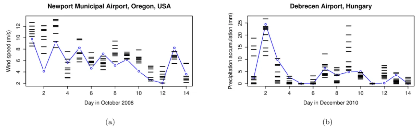
Figure 1.1: (a) Wind speed observations (blue line) and corresponding UWME forecasts (bars) for Newport Municipal Airport, Oregon, USA, for the first two weeks of October 2008; (b) observed precipitation accumulation (blue line) and the corresponding ALADIN- HUNEPS ensemble forecasts (bars) for Debrecen Airport, Hungary, for the first two weeks of December 2010.

Although the transition from single deterministic forecasts to ensemble predictions can be seen as an important step towards probabilistic forecasting, ensemble forecasts are often underdispersive, that is, the spread of the ensemble is too small to account for the full uncertainty, and subject to systematic bias. This phenomenon has been observed with several operational ensemble prediction systems (see e.g. Buizza et al., 2005; Park et al., 2008; Bougeault et al., 2010). A possible solution to account for this deficiency is some form of statistical post-processing (Buizza, 2018).

To illustrate the systematic errors of ensemble forecasts, Figure 1.1a shows UWME wind speed forecasts for Newport Municipal Airport (OR) and the corresponding observations for the first two weeks of October 2008, and Figure 1.1b shows ALADIN-HUNEPS forecasts of precipitation accumulation at Debrecen Airport and the corresponding observations for the first two weeks of December 2010. Both time series illustrate the lack of an appropriate representation of the forecast uncertainty as the verifying observations frequently fall outside the range of the ensemble forecasts.

1.2 Statistical post-processing

Over the past decade, various statistical post-processing methods have been proposed in the meteorological and statistical literature, for an overview see e.g. Wilks (2006); Gneit- ing (2014); Williams et al.(2014), or Vannitsemet al.(2018). Among these probably the most popular parametric approaches are the BMA (Raftery et al., 2005) and the EMOS or non-homogeneous regression (Gneiting et al., 2005), which are partially implemented in the ensembleBMA (Fraley et al., 2011) and ensembleMOS (Yuen et al., 2018) packages of R (R Core Team, 2019) and provide estimates of the probability distributions of the predictable weather quantities. Once the predictive distribution is given, its functionals (e.g. median or mean) can easily be calculated and considered as point forecasts.

The BMA predictive probability density function (PDF) of a future weather quantity is the weighted sum of individual PDFs corresponding to the ensemble members. An individual PDF can be interpreted as the conditional PDF of the future weather quantity

(13)

1.2. STATISTICAL POST-PROCESSING 5 provided the considered forecast is the best one and the weights are based on the relative performance of the ensemble members during a given training period. In this way BMA is a special, fixed parameter version of dynamic model averaging method developed by Raftery et al. (2010). Weights and other model parameters are usually estimated using linear regression and ML method, where the maximum of the likelihood function is found by the EM algorithm. We remark that due to their flexibility, mixture models play an essential role in data analysis (B¨ohning, 2014) and parameter estimation in mixture models is a typical application of the EM algorithm (see Dempster et al. (1977), McLachlan and Krishnan (1997) or more recently Lee and Scott (2012), Chen and Lindsay (2014)).

The BMA models of various weather quantities differ only in the PDFs of the mixture components. For temperature and sea level pressure a normal distribution provides an appropriate model (Raftery et al., 2005), but different laws are needed for wind speed (Sloughteret al., 2010; Baran, 2014), precipitation (Sloughteret al., 2007) or surface wind direction (Bao et al., 2010). However, one should also mention that in some situations BMA post-processing might result, for instance, in model overfitting (Hamill, 2007) or overweighting climatology (Hodyss et al., 2016).

The essentially simpler EMOS approach uses a single parametric distribution as a predictive PDF with parameters depending on the ensemble members. The unknown parameters specifying this dependence are estimated using forecasts and validating observations from a rolling training period, which allows automatic adjustments of the statistical model to any changes of the EPS (for instance seasonal variations or EPS model updates). Similar to the BMA approach, different weather quantities require different predictive PDFs. For example, Gneiting et al. (2005) models temperature with a Gaus- sian predictive distribution where the mean is an affine function of the ensemble member forecasts and the variance is an affine function of the ensemble variance. Over the last years the EMOS approach has been extended to other weather variables such as wind speed (Thorarinsdottir and Gneiting, 2010; Lerch and Thorarinsdottir, 2013; Baran and Lerch, 2015; Scheuerer and M¨oller, 2015), precipitation (Scheuerer, 2014; Scheuerer and Hamill, 2015; Baran and Nemoda, 2016), and total cloud cover (Hemriet al., 2016).

To illustrate the EMOS approach to post-processing, Figure 1.2a shows the observed wind speed, the corresponding UWME forecasts and truncated normal (TN) and log- normal (LN) EMOS predictive distributions (for details see Sections 3.2.1 and 3.2.2, respectively) for Newport Municipal Airport for 2 October 2008. A different situation is shown in Figure 1.2b, where the observed precipitation accumulation, the corresponding ALADIN-HUNEPS ensemble forecasts and estimated censored and shifted gamma (CSG) and censored generalized extreme value (GEV) EMOS predictive distributions (see Sec- tions 4.2.1 and 4.2.2, respectively) for Debrecen Airport for 12 December 2010 are plotted.

In both cases, the spread of the ensemble forecasts is notably smaller than the spread of the post-processed forecast distribution. Note that in both examples two different EMOS models are proposed for the same weather quantity and in general, the success of statistical post-processing relies on finding appropriate parametric families for the weather variable of interest. However, the choice of a suitable parametric model is a non-trivial task and often a multitude of competing models is available. The relative performances of these models usually vary for different data sets and applications.

The regime-switching combination models proposed by Lerch and Thorarinsdottir (2013) and also investigated by Baran and Lerch (2015) partly alleviate the limited flexibility of single parametric family models by selecting one of several candidate models

(14)

6 CHAPTER 1. PROBABILISTIC FORECASTS AND FORECAST EVALUATION

0 5 10 15

0.000.050.100.15

Newport Municipal Airport (OR), 2 October 2008

Wind speed (m/s)

Density

TN EMOS LN EMOS

0 5 10 15

0.000.050.100.150.20

Debrecen Airport, 12 December 2010

Precipitation accumulation (mm)

Density

CSG EMOS GEV EMOS

(a) (b)

Figure 1.2: (a) Wind speed observations, the corresponding UWME forecasts and TN and LN EMOS predictive distributions for Newport Municipal Airport (OR) for 2 Octo- ber 2008; (b) observed precipitation accumulation, the corresponding ALADIN-HUNEPS ensemble forecasts and CSG and GEV EMOS predictive distributions for Debrecen Air- port for 12 December 2010. Ensemble members: red bars; ensemble median: vertical red line; observation: vertical orange line; predictive PDFs: blue/green lines; EMOS medians:

vertical blue/green lines.

based on covariate information. However, the applicability of this approach is subject to the availability of suitable covariates. For some weather variables, full mixture EMOS models can be formulated where the parameters and weights of a mixture of two forecast distributions are estimated jointly (Baran and Lerch, 2016). However, such approaches are limited to specific weather variables, and the estimation is computationally demanding.

Recently a more generally applicable route towards improving the forecast performance has received significant interest (see e.g. M¨oller and Groß, 2016; Yang et al., 2017;

Bassettiet al., 2018), which is based on a two-step combination of predictive distributions from individual post-processing models. In the first step, individual EMOS models based on single parametric distributions are estimated, whereas in the second step the forecast distributions are combined utilizing state of the art forecast combination techniques such as the (spread-adjusted) linear pool, the beta-transformed linear pool (Gneiting and Ranjan, 2013), or the recently proposed Bayesian, essentially non-parametric calibration approach (Bassettiet al., 2018). Besides these techniques Baran and Lerch (2018) propose a computationally efficient ’plug-in’ approach to determining combination weights in the linear pool that is specific to post-processing applications.

Besides the calibration of univariate weather quantities an increasing interest has appeared in modelling correlations between the different weather variables. In the special case of wind vectors, Pinson (2012) suggested an adaptive calibration technique, whereas Schuhen et al. (2012) and Sloughter et al. (2013) introduced bivariate EMOS and BMA models, respectively. Further, Möller et al. (2013) developed a general approach where after univariate calibration of the weather variables, the component predictive PDFs are joined into a multivariate predictive density with the help of a Gaussian copula. An- other idea appears in the ensemble copula coupling method Schefzik et al. (2013), where after univariate calibration the rank order information in the raw ensemble is used to restore correlations. For joint post-processing of ensemble forecasts of wind speed and temperature Baran and Möller (2015) and Baran and Möller (2017) propose bivariate

(15)

1.3. POST-PROCESSING APPROACHES 7 BMA and EMOS models, respectively, and finally, Schefzik (2016a,b) introduces non- parametric approaches for modelling spatial dependencies between individual univariate and multivariate post-processed forecasts.

Statistical calibration can also be applied to improve the performance of hydrological forecasts. EMOS based statistical post-processing turned out to improve the predictive performance of hydrological ensemble forecasts for different gauges along river Rhine (Hemri et al., 2015; Hemri and Klein, 2017), whereas Baran et al. (2019a) propose a doubly truncated BMA model for calibration of Box-Cox transformed ensemble forecasts of water levels.

1.3 Post-processing approaches

As mentioned in Section 1.2, the Bayesian model averaging and ensemble model output statistics are among the most popular post-processing approaches as they provide full predictive distributions. In the present work we also concentrate on various versions of these techniques describing new models and applications.

In what follows, let f₁, f₂, . . . , f_K denote the ensemble forecast of a given weather or hydrological quantity X for a given location, time and lead time under the assumption that the ensemble members can be clearly distinguished and they are not exchangeable.

Such forecasts are usually outputs of multi-model, multi-analyses EPSs, where each member can be identified and tracked. This property holds e.g. for the UWME or for the COSMO-DE ensemble.

However, recently most operational EPSs incorporate ensembles where at least some members can be considered as statistically indistinguishable and in this way exchangeable, as these forecasts are generated using perturbed initial conditions. This is the case with the 51-member operational ECMWF ensemble or one can mention multi-model EPSs such as the Grand Limited Area Model Ensemble Prediction System (GLAMEPS) ensemble (Iversen et al., 2011) or the THORPEX² Interactive Grand Global Ensemble (Swinbank et al., 2016).

In the remaining part of this chapter, if we have M ensemble members divided into K exchangeable groups, where the kth group contains M_k ≥ 1 ensemble members (PK

k=1M_k=M), notation f_k,` is used for the `th member of the kth group.

1.3.1 Bayesian model averaging

The BMA predictive distribution of a weather or hydrological quantity X for a given location, time and lead time proposed by Rafteryet al. (2005) is a weighted mixture with PDF

p(x|f₁, . . . , f_K;θ₁, . . . , θ_K) :=

K

X

k=1

ω_kg x|f_k, θ_k

, (1.3.1)

where g x|fk, θk

is the component PDF from a parametric family corresponding to the kth ensemble member f_k with parameter (vector) θ_k to be estimated, and ω_k is the corresponding weight determined by the relative performance of this particular member

2The Observing System Research and Predictability Experiment

(16)

8 CHAPTER 1. PROBABILISTIC FORECASTS AND FORECAST EVALUATION during the training period. Note that the weights should form a probability distribution, that is ω_k≥0, k = 1,2, . . . , K, and PK

k=1ω_k= 1.

To account for the existence of groups of exchangeable ensemble members, Fraley et al. (2010) suggest to use the same weights and parameters within a given group. Thus, if we have M ensemble members divided into K exchangeable groups, model (1.3.1) is replaced by

p(x|f_1,1, . . . , f_1,M₁, . . . , f_K,1, . . . , f_K,M_K;θ₁, . . . , θ_K) :=

K

X

k=1 M_k

X

`=1

ω_kg x|f_k,`, θ_k

. (1.3.2) For the sake of simplicity, in Sections 2.1, 3.1, 4.1 and 5.1 we provide results and formulae only for model (1.3.1) as their extension to model (1.3.2) is rather straightforward.

Model parameters θ_k and weights ω_k, k = 1,2, . . . , K, are usually estimated using rolling training data consisting of ensemble members and verifying observations from the preceding n days. In general, a maximum likelihood approach is applied.

BMA models corresponding to various weather or hydrological quantities differ in the component parametric distribution families and in the way the parameters are linked to the ensemble members. E.g. to model temperature and sea level pressure Raftery et al.

(2005) propose a normal mixture with predictive distribution of the form

K

X

k=1

ω_kN α_k+β_kf_k, σ² ,

other currently available models with the corresponding quantities to be forecast are listed below.

• Wind speed:

– Gamma mixture (Sloughteret al., 2010), for details see Section 3.1.1;

– Truncated normal mixture with cut-off at 0 from below (Baran, 2014), for details see Section 3.1.2.

• Precipitation accumulation:

– Discrete-continuous model. Point mass at zero, gamma mixture for modelling positive precipitation accumulation (Sloughteret al., 2007), for details see Sec- tion 4.1.

• Wind direction:

– Von-Mises mixture (Bao et al., 2010).

• Box-Cox transformed water levels:

– Doubly truncated normal mixture (Baranet al., 2019a), for details see Section 2.1

• Wind vector:

– Bivariate normal mixture (Sloughter et al., 2013).

(17)

1.3. POST-PROCESSING APPROACHES 9

• Wind speed and temperature:

– Bivariate normal mixture truncated from below at zero in the wind coordinate (Baran and M¨oller, 2015), for details see Section 5.1.

1.3.2 Ensemble model output statistics

In contrast to the BMA approach, the EMOS forecast distribution is given by a single parametric law with parameters that depend on the ensemble forecast. For a given weather or hydrological quantity X for a given location, time and lead time it has the general form

X |f₁, . . . , f_K ∼h(x|f₁, . . . , f_K;θ),

where the parametric PDF h(x|f₁, . . . , f_K;θ) is connected to the ensemble members with the help of suitable link functions. E.g. the EMOS predictive distribution for temperature and sea level pressure suggested by Gneiting et al. (2005) is

N a₀ +a₁f₁+. . .+a_Kf_K, b₀+b₁S²

with S² := 1 K−1

K

X

k=1

f_k−f2

, (1.3.3) where f denotes the ensemble mean.

If the ensemble contains groups of statistically indistinguishable ensemble members, members within a given group should share the same parameters (Gneiting, 2014) resulting in the exchangeable version

N a₀+a₁f₁+· · ·+a_Kf_K, b₀+b₁S² of model (1.3.3), where f_k denotes the mean of the kth group.

Parameters of an EMOS model are estimated by optimizing the mean value of a proper scoring rule (see Section 1.4) over the forecast cases in the (usually rolling) training data.

Again, different weather or hydrological quantities require different predictive distributions and link functions.

• Wind speed:

– Truncated normal distribution with cut-off at 0 from below (Thorarinsdottir and Gneiting, 2010), for details see Section 3.2.1;

– Generalized extreme value distribution (Lerch and Thorarinsdottir, 2013), for details see Section 3.2.3;

– Log-normal distribution (Baran and Lerch, 2015), for details see Section 3.2.2.

• Precipitation accumulation:

– Censored generalized extreme value distribution (Scheuerer, 2014), for details see Section 4.2.2;

– Censored, shifted gamma distribution (Scheuerer and Hamill, 2015; Baran and Nemoda, 2016), for details see Section 4.2.1.

• Box-Cox transformed water levels:

(18)

10 CHAPTER 1. PROBABILISTIC FORECASTS AND FORECAST EVALUATION – Doubly truncated normal distribution (Hemri et al., 2015; Hemri and Klein,

2017), for details see Section 2.2.

• Wind vector:

– Bivariate normal distribution (Schuhenet al., 2012).

• Wind speed and temperature:

– Bivariate normal distribution truncated from below at zero in the wind coordinate (Baran and M¨oller, 2017), for details see Section 5.2.

1.3.3 Parameter estimation strategies

The choice of the training data is important for statistical post-processing. As mentioned before, for estimating the BMA and EMOS model parameters usually a rolling training period is applied, and the estimates are obtained using ensemble forecasts and corresponding validating observations for the preceding n calendar days. Given a training period, there are two traditional approaches for spatial selection of the training data (Thorarins- dottir and Gneiting, 2010). In the global (regional) approach, parameters are estimated using all available forecast cases from the training period resulting in a single universal set of parameters across the entire ensemble domain. It requires quite short training periods (see e.g. Baran et al. (2013, 2014a,b) and Baran and Nemoda (2016), where the optimal training period lengths for ALADIN-HUNEPS wind speed, temperature and precipitation forecasts are given), but usually it is unsuitable for large and heterogeneous observation domains. For local parameter estimation, one has distinct parameter estimates for the different stations obtained using only training data of the given station. To avoid numerical stability problems, local models require much longer training periods (for optimal training period lengths for EMOS modelling of different weather quantities see e.g. Hemri et al., 2014), but if the training data is large enough, it will usually outperform the regional approach. To combine the advantages of local and regional estimation, Lerch and Baran (2017) introduced two semi-local methods where the training data for a given station is augmented with data from stations with similar characteristics. The choice of similar stations is based either on suitably defined distance functions or on clustering. In the distance based approach, which generalizes the idea of Hamill et al. (2008), training sets of a given station are increased by including training data from the L nearest stations, and distances are measured from historical data. In the clustering based semi-local method, the observation sites are grouped into clusters using k-means clustering of feature vectors depending both on the station climatology (observations at the given station) and the forecast errors of the raw ensemble during the training period, then a regional parameter estimation is performed within each cluster. With the help of these methods one can get reliable parameter estimates even for short training periods and the obtained models may outperform the local BMA or EMOS approaches (Lerch and Baran, 2017). A detailed description of semi-local approaches to parameter estimation can be found in Chapter 6.

(19)

1.4. FORECAST EVALUATION 11

1.4 Forecast evaluation

In probabilistic forecasting the general aim is to access the maximal sharpness of the predictive distribution subject to calibration (Gneiting et al., 2007), where the latter means a statistical consistency between the predictive distributions and the validating observations, whereas the former refers to the concentration of the predictive distribution.

One of the simplest tools for getting a first impression about the calibration of ensemble forecasts is the verification rank histogram (or Talagrand diagram), defined as the histogram of ranks of validating observations with respect to the corresponding ensemble forecasts (see e.g. Wilks, 2011, Section 8.7.2). In the case of a properly calibrated K- member ensemble, the ranks follow a uniform distribution on {1,2, . . . , K+ 1}, and the deviation from uniformity can be quantified by the reliability index ∆ defined by

∆ :=

K+1

X

r=1

ρ_r− 1 K+ 1

, (1.4.1)

where ρ_r is the relative frequency of rank r (Delle Monacheet al., 2006). The verification rank histogram can also be generalized to multivariate ensemble forecasts, however, in this case the usual problem is the proper definition of ranks. In Chapter 5 of the present work we use the multivariate ordering proposed by Gneiting et al. (2008). For a probabilistic forecast one can calculate the reliability index (and plot the verification rank histogram as well) from a preferably large number of ensembles sampled from the predictive PDF and the corresponding verifying observations.

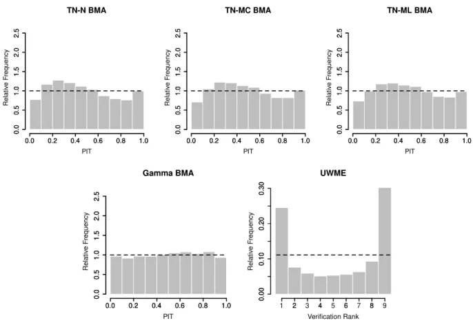
In the univariate case the continuous counterpart of the verification rank histogram is the probability integral transform (PIT) histogram. By definition, the PIT is the value of predictive cumulative distribution function (CDF) at the validating observation (Raftery et al., 2005), which in case of proper calibration should follow a uniform distribution on the [0,1] interval. Apart from the visual inspection of PIT histograms, formal statistical test of uniformity can be used to assess calibration. The simplest idea is to make use of the Kolmogorov-Smirnov test. This approach is followed in the case study of Section 2.3. However, as the PIT values of multi-step ahead probabilistic forecast exhibit se- rial correlation (see e.g. Diebold et al., 1998) and the probabilistic forecasts cannot be assumed to be independent in space and time, one can employ a moment-based test of uniformity proposed by Kn¨uppel (2015), which accounts for dependence in the PIT values. In particular, in Sections 3.3 and 4.3 we use theα⁰₁₂₃₄ test of Kn¨uppel (2015) that has been demonstrated to have superior size and power properties compared with alternative choices.

Predictive performance can be quantified with the help of scoring rules, which are loss functions S(F, x) assigning numerical values to pairs (F, x) of forecasts and observations.

In the atmospheric sciences the most popular scoring rules are the continuous ranked probability score (CRPS; Gneiting and Raftery, 2007; Wilks, 2011) and the logarithmic score (LogS; Good, 1952). For a (predictive) CDF F(y) and real value (observation) x the CRPS is defined as

CRPS F, x :=

Z ∞

−∞

F(y)−I{y≥x}

2

dy= Z x

−∞

F²(y)dy+ Z ∞

x

1−F(y)2

dy (1.4.2)

=E|X−x| −1

2E|X−X⁰|,

(20)

12 CHAPTER 1. PROBABILISTIC FORECASTS AND FORECAST EVALUATION where IH denotes the indicator of a set H, whereas X and X⁰ are independent random variables with CDF F and finite first moment. The last representation in (1.4.2) implies that the CRPS can be expressed in the same unit as the observation. In most applications the CRPS has a simple closed form (see e.g. the R package scoringRules;

Jordan et al., 2017), otherwise the second integral expression in the definition (1.4.2) should be evaluated numerically. According to our tests with the mixture EMOS model of Section 3.2.5 (see also Baran and Lerch, 2016), this approach results in slightly more accurate results and faster calculations than the numerical evaluation of the first integral defining the CRPS. The logarithmic score is the negative logarithm of the predictive density f(y) evaluated at the verifying observation, i.e.,

LogS(F, x) :=−log(f(x)). (1.4.3)

Both CRPS and LogS are proper scoring rules (Gneiting and Raftery, 2007) which are negatively oriented, that is, smaller scores indicate better forecasts.

A direct multivariate extension of the CRPS is the energy score (ES) introduced by Gneiting and Raftery (2007). Given a CDF F on R^d and a d-dimensional vector x, the energy score is defined as

ES(F,x) := EkX−xk − 1

2EkX−X⁰k, (1.4.4)

where k · k denotes the Euclidean distance and, similar to the univariate case, X and X⁰ are independent random vectors having distribution F. However, in most cases (see Section 5.4) the ES cannot be given in a closed form, so it is replaced by a Monte Carlo approximation

ES(F,c x) := 1 n

n

X

j=1

kX_j −xk − 1 2(n−1)

n−1

X

j=1

kX_j−X_j+1k, (1.4.5)

where X1,X2, . . . ,Xn is a large random sample from F (Gneitinget al., 2008). Finally, if F is a CDF corresponding to a forecast ensemble f₁,f₂, . . . ,f_K then (1.4.5) reduces to

ES(F,x) = 1 K

K

X

j=1

kf_j−xk − 1 2K²

K

X

j=1 K

X

k=1

kf_j −f_kk. (1.4.6) Obviously, for univariate quantities (1.4.5) and (1.4.6) result in the approximation of the CRPS of a probabilistic forecast and CRPS of the raw ensemble, respectively.

Besides the CRPS one can also consider Brier scores (BS; Wilks, 2011, Section 8.4.2) for the dichotomous event that the observation x exceeds a given threshold y. For a predictive CDF F(y) the Brier score is defined as

BS F, x;y

:= F(y)−I^{y≥x}2

, (1.4.7)

(see e.g. Gneiting and Ranjan, 2011), and note that the CRPS is the integral of the BS over all possible thresholds. Brier score is also negatively oriented and it plays an important role e.g. in evaluating forecasts of the probability of no precipitation.

(21)

1.4. FORECAST EVALUATION 13 To evaluate the goodness of fit of probabilistic forecasts to extreme values of the univariate weather quantity at hand, a useful tool to be considered is the threshold- weighted continuous ranked probability score (twCRPS)

twCRPS F, x :=

Z ∞

−∞

F(y)−I{y≥x}

2

ω(y)dy (1.4.8)

introduced by Gneiting and Ranjan (2011), where ω(y) ≥ 0 is a weight function. Ob- viously, ω(y) ≡ 1 corresponds to the traditional CRPS defined by (1.4.2), while to address values of the studied weather variable above a given threshold r one may set ω(y) =I{y≥r}. In the case studies of Chapter 3 we consider threshold values corresponding approximately to the 90th, 95th and 98th percentiles of the wind speed observations.

In case studies, with respect to a given score S(F, x), competing forecast methods can be compared by the mean score value

S_F := 1 N

N

X

i=1

S F_i, x_i

(1.4.9) over all pairs (F_i, x_i), i = 1,2, . . . , N, of forecasts and observations in the verification data. Further, the improvement in a score S_F for a forecast F with respect to a reference forecast Fref can be quantified with the help of the corresponding skill score (Gneiting and Raftery, 2007), defined as

S_F^skill := 1− SF

SF_ref

, (1.4.10)

where S_F_ref denotes the mean score value corresponding to the reference approach. Thus, besides the CRPS, BS and twCRPS one can also investigate the continuous ranked probability skill score (CRPSS; see e.g. Murphy, 1973; Gneiting and Raftery, 2007), the Brier skill score (BSS; see e.g. Friedrichs and Thorarinsdottir, 2012) and the threshold-weighted continuous ranked probability skill score (twCRPSS; see e.g. Lerch and Thorarinsdottir, 2013), respectively. These scores are positively oriented, that is the larger the better. In the case studies of Chapters 2 and 4 we use the raw ensemble as a reference, whereas in Chapter 3 skill scores with respect to the TN EMOS model are reported.

To compare the calibration of probabilities of a dichotomous event of exceeding a given threshold calculated from the raw ensemble and the BMA and EMOS predictive distributions, one can make use of reliability diagrams (Wilks, 2011, Section 8.4.4). The reliability diagram plots the a graph of the observed frequency of the event against the binned forecast frequencies and in the ideal case this graph should lie on the main diagonal of the unit square. In the case studies of Chapter 4 the same thresholds as for the BSs are considered, whereas the unit interval is divided into 11 bins with break points 0.05,0.15,0.25, . . . ,0.95. Following Br¨ocker and Smith (2007) and Scheuerer (2014), the observed relative frequency of a bin is plotted against the mean of the corresponding probabilities, and inset histograms displaying the frequencies of the different bins on log 10 scales are also added.

Calibration and sharpness of a univariate predictive distribution can also be investigated using the coverage and average width of the (1−α)100 %, α ∈ (0,1), central prediction interval, respectively. As coverage we consider the proportion of validating

(22)

14 CHAPTER 1. PROBABILISTIC FORECASTS AND FORECAST EVALUATION observations located between the lower and upper α/2 quantiles of the predictive CDF, and level α should be chosen to match the nominal coverage of the raw ensemble, that is (K −1)/(K + 1)100%, where again K is the ensemble size. As the coverage of a calibrated predictive distribution should be around (1−α)100 %, such a choice of α allows direct comparison with the raw ensemble.

However, sharpness of an ensemble forecast or of a predictive distribution can also be quantified by its standard deviation. An obvious generalization of this idea to d- dimensional quantities is the determinant sharpness (DS; M¨oller et al., 2013) defined as

DS := det(Σ)1/(2d)

, (1.4.11)

where Σ is the covariance matrix of an ensemble or of a predictive PDF.

As point forecasts one can consider median and mean of the raw ensemble and of the calibrated predictive distribution, which in the univariate case are evaluated with the use of mean absolute errors (MAEs) and root mean square errors (RMSEs). Note that MAE optimal for the median, while RMSE is optimal for the mean forecasts (Gneiting, 2011; Pinson and Hagedorn, 2012). For multivariate point forecasts the RMSE should be replaced by the mean Euclidean error (EE) of forecasts from the corresponding validating observations, where the ensemble median can be obtained using the Newton-type algorithm given in Dennis and Schnabel (1983), the algorithm of Vardi and Zhang (2000), or any other method implemented, e.g. in the R package pcaPP (Fritz et al., 2012). For a predictive distribution F one may apply the same algorithm on a preferably large sample from F.

Finally, as suggested by Gneiting and Ranjan (2011), statistical significance of the differences between the verification scores is assessed by utilizing the Diebold-Mariano (DM;

Diebold and Mariano, 1995) test, which allows accounting for the temporal dependencies in the forecast errors. Given a scoring rule S and two competing probabilistic forecasts F and G, let

di(F, G) :=S(Fi, xi)− S(Gi, xi), i= 1,2, . . . , N,

denote the score differences over the verification data of size N. The test statistic of the DM test is given by

t_N =√

NS_F − S_G

σb_N , (1.4.12)

where S_F and S_G are the mean scores (1.4.9) corresponding to forecasts F and G, respectively, and bσN is a suitable estimator of the asymptotic standard deviation of the sequence of score differences d_i(F, G). Under some weak regularity assumptions, t_N asymptotically follows a standard normal distribution under the null hypothesis of equal predictive performance. Negative values of tN indicate a better predictive performance of F, whereas G is preferred in case of positive values of t_N. In the case studies of Chapters 2–5, following suggestions of Diebold and Mariano (1995) and Gneiting and Ranjan (2011), as an estimator bσN in (1.4.12) for h step ahead forecasts we use the sample autocovariance up to lag h−1.

(23)

Chapter 2 Statistical post-processing of hydrological ensemble forecasts

Hydrological forecasts are important for a heterogeneous group of users such as, for instance, the operators of hydrological power plants, flood prevention authorities, or ship- ping companies. For rational decision making based on cost-benefit analyses an estimate of the predictive uncertainty (Krzysztofowicz, 1999; Todini, 2008) needs to be provided with any forecast. The state of the art approach of using a set of parallel runs of a hydrological model driven by meteorological ensemble forecasts provided by NWP models (Cloke and Pappenberger, 2009) gives a first estimate of the meteorological input uncertainty. How- ever, as mentioned in Section 1.1, NWP ensembles are usually biased and underdispersed and other sources of uncertainty like hydrological model formulation, boundary and initial condition uncertainty as well as measurement uncertainties are typically neglected.

Hence, statistical post-processing is important in order to reduce systematic errors and to obtain an appropriate estimate of the predictive uncertainty. In this chapter, which is based on Baran et al.(2019a), we introduce a novel BMA approach to post-processing hydrological ensemble forecast and in a case study dealing with water levels at gauge Kaub of river Rhine, the forecast skill of this new model is compared with the predictive performance of the recently developed EMOS method of Hemri and Klein (2017) and the raw ensemble forecasts.

2.1 Doubly truncated normal BMA model

For weather variables such as temperature or pressure, BMA models with Gaussian components provide a reasonable fit (Rafteryet al., 2005; Fraleyet al., 2010), however, water levels are typically non-Gaussian (see e.g. Duanet al., 2007), moreover, they are bounded both from below and from above. These constraints should also be taken into account during model formulation. A general procedure is to normalize the forecasts and observations using, for instance, Box-Cox transformation

h_λ(x) :=

( x^λ−1

/λ, λ6= 0,

log(x), λ= 0 (2.1.1)

with some coefficient λ, perform post-processing, and then back-transform the results using the inverse Box-Cox transformation (Duan et al., 2007; Hemri et al., 2013, 2014,

(24)

16 CHAPTER 2. POST-PROCESSING OF HYDROLOGICAL FORECASTS 2015).

2.1.1 Model formulation

In Duanet al.(2007) and Hemri et al.(2013) the Box-Cox transformation is used prior to applying BMA in order to achieve approximate normality despite the positive skewness of water levels. Additionally, it is important to ensure that the resulting water level quantiles of the predictive distribution are within realistic physical bounds. At the upper bound of the distribution water levels should be lower than a water level threshold resulting from an extreme flood with a small exceedance probability, at the lower bound water levels should be higher than a water level threshold resulting from an extreme long-lasting low water period with a small non-exceedance probability. In order to ensure realistic values while still being able to benefit from the mathematical simplicity of Gaussian models, following the ideas of Hemri and Klein (2017), for modelling Box-Cox transformed water levels we use a doubly truncated normal distribution N_a^b µ, σ²

, with PDF ga,b x|µ, σ

:=

1

σϕ ^x−µ_σ Φ ^b−µ_σ

−Φ ^a−µ_σ , x∈[a, b], (2.1.2) and ga,b x|µ, σ

:= 0, otherwise, where a and b are the lower and upper bounds and ϕ and Φ denote the PDF and the CDF of the standard normal distribution, respectively.

Note that the mean and variance of N_a^b µ, σ² are κ =µ+σϕ ^a−µ_σ

−ϕ ^b−µ_σ Φ ^b−µ_σ

−Φ ^a−µ_σ and (2.1.3)

%² =σ²



1 +

a−µ

σ ϕ ^a−µ_σ

− ^b−µ_σ ϕ ^b−µ_σ Φ ^b−µ_σ

−Φ ^a−µ_σ − ϕ ^a−µ_σ

−ϕ ^b−µ_σ Φ ^b−µ_σ

−Φ ^a−µ_σ

!2

,

respectively. The proposed BMA predictive PDF (Baran et al., 2019a) is p x|f₁, . . . , f_K;β₀₁, . . . , β_0K;β₁₁, . . . , β_1K;σ

=

K

X

k=1

ω_kg_a,b x|β_0k+β_1kf_k, σ

, (2.1.4) where we assume that the location of the kth mixture component is an affine function of the corresponding ensemble memberf_k, and scale parameters are assumed to be equal for all component PDFs. The latter assumption is for the sake of simplicity and is common in BMA modelling (see e.g. Rafteryet al., 2005), whereas the form of the location parameter is in line with the truncated normal BMA model of Baran (2014), see also Section 3.1.2.

Further, note that the EMOS model of Hemri and Klein (2017) (see Section 2.2) also links the ensemble members to the location and scale of the truncated normal distribution and not to the corresponding mean and variance.

2.1.2 Parameter estimation

Location parameters β_0k, β_1k, weights ω_k, k= 1,2, . . . , K, and scale parameter σ can be estimated from training data, which consists, for instance, of ensemble members and

(25)

2.1. DOUBLY TRUNCATED NORMAL BMA MODEL 17 validating observations from the preceding n days. In the BMA approach, estimates of location parameters are typically obtained by regressing the validating observations on the ensemble members, whereas weights and scale parameter(s) are obtained via ML estimation (see e.g. Rafteryet al., 2005; Sloughteret al., 2007, 2010), where the log-likelihood function of the training data is maximized using the EM algorithm for mixture distributions (Dempster et al., 1977; McLachlan and Krishnan, 1997). However, the regression approach assumes the location parameters to be simple functions of the mean, which is obviously not the case for the truncated normal distribution, see (2.1.3). Hence, we propose a pure ML method estimating all model parameters by maximizing the likelihood function, which idea has already been considered e.g. by Sloughter et al.(2010).

In what follows, for a given location s∈ S and time t∈ T let f_k,s,t denote the kth ensemble member, and denote by x_s,t the corresponding validating observation. Here S denotes the set of locations sharing the same BMA model parameters and T is the set of training dates. In the case study of Section 2.3, S consists of a single location, however, for more complex ensemble domains different choices of training data are possible, for more details see Chapter 6. Further, as in the case study of Section 2.3 the different lead times are treated separately, reference to the lead time of the forecast is omitted. By assuming the conditional independence of forecast errors with respect to the ensemble members in space and time, the log-likelihood function for model (2.1.4) corresponding to all forecast cases (s, t) in the training set equals

`(ω₁, . . . , ω_K, β₀₁, . . . , β_0K, β₁₁, . . . , β_1K, σ) = X

s,t

log

" _K X

k=1

ω_kg_a,b x_s,t|β_0k+β_1kf_k,s,t, σ

# . (2.1.5) To obtain the ML estimates we apply EM algorithm for truncated Gaussian mixtures proposed by Lee and Scott (2012) with a mean correction. In line with the classical EM algorithm for mixtures (McLachlan and Krishnan, 1997), first we introduce latent binary indicator variables z_k,s,t identifying the mixture component where the observation x_s,t comes from, that is z_k,s,t is one or zero according as whether x_s,t follows or not the kth component distribution. Using these indicator variables one can provide the complete data log-likelihood corresponding to (2.1.5) in the form

`_C(ω₁, . . . , ω_K, β₀₁, . . . , β_0K, β₁₁, . . . , β_1K, σ) (2.1.6)

=X

s,t K

X

k=1

z_k,s,th

log ω_k

+ log

g_a,b x_s,t|µ_k,s,t, σi ,

with µ_k,s,t := β_0k+β_1kf_k,s,t. After specifying the initial values of the parameters the EM algorithm alternates between an expectation (E) and a maximization (M) step until convergence. As first guesses β_0k⁽⁰⁾ and β_1k⁽⁰⁾, k = 1,2, . . . , K, for the location parameters we suggest to use the coefficients of the linear regression of x_s,t on f_k,s,t, so µ⁽⁰⁾_k,s,t = β_0k⁽⁰⁾+β_1k⁽⁰⁾f_k,s,t. Initial scale σ⁽⁰⁾ can be the standard deviation of the observations in the training data set or the average residual standard deviation from the above regression, whereas the initial weights might be chosen uniformly, that is ω_k⁽⁰⁾ = 1/K, k = 1,2, . . . , K.

Then in the E step the latent variables are estimated using the conditional expectation of the complete log-likelihood on the observed data, while in the M step the parameter estimates are updated by maximizing `_C given the actual values of the latent variables.