arXiv:1604.02746v2 [math.CO] 11 Aug 2017
Properties of minimally t-tough graphs
Gyula Y. Katona
∗1, Dániel Soltész
†2, and Kitti Varga
‡31,2,3
Department of Computer Science and Information Theory, Budapest University of Technology and Economics
1
MTA-ELTE Numerical Analysis and Large Networks Research Group
August 14, 2017
Abstract
A graph G is minimally t-tough if the toughness of G is t and the deletion of any edge from G decreases the toughness. Kriesell conjectured that for every minimally 1-tough graph the minimum de- gree δ(G) = 2. We show that in every minimally 1-tough graph δ(G) ≤ n3 + 1. We also prove that every minimally1-tough, claw-free graph is a cycle. On the other hand, we show that for every positive rational numbertany graph can be embedded as an induced subgraph into a minimally t-tough graph.
1 Introduction
All graphs considered in this paper are finite, simple and undirected. Letd(v) denote the degree of a vertexv,ω(G)denote the number of components,α(G) denote the independence number and δ(G) denote the minimum degree of a graph G.
Definition 1.1. A graph G is k-connected, if it has at least k + 1 vertices and remains connected whenever fewer than k vertices are removed. The connectivity ofG, denoted byκ(G), is the largest k for whichGisk-connected.
∗kiskat@cs.bme.hu
†solteszd@math.bme.hu
‡vkitti@cs.bme.hu
The more edges a graph has, the larger its connectivity can be, so the graphs, which are k-connected and have the fewest edges for this property, may be interesting.
Definition 1.2. A graph G is minimally k-connected, if κ(G) = k and κ(G−e)< k for all e∈E(G).
Clearly, all degrees of a k-connected graph have to be at least k. On the other hand, Mader proved that the minimum degree of every minimally k-connected graph is exactly k.
Theorem 1.3 (Mader [7]). Every minimallyk-connected graph has a vertex of degree k.
The notion of toughness was introduced by Chvátal [3] in 1973.
Definition 1.4. Lett be a positive real number. A graph Gis called t-tough, if ω(G−S)≤ |S|/t for any cutset S of G. The toughness of G, denoted by τ(G), is the largest t for which G ist-tough, takingτ(Kn) =∞for all n≥1.
We say that a cutset S ⊆V(G) is a tough set if ω(G−S) =|S|/τ(G).
We can define an analogue of minimallyk-connected graphs for the notion of toughness.
Definition 1.5. A graph G is said to be minimally t-tough, if τ(G) =t and τ(G−e)< t for all e∈E(G).
It follows directly from the definition that every t-tough graph is 2t- connected, implying κ(G) ≥ 2τ(G) for noncomplete graphs. Therefore, the minimum degree of any 1-tough graph is at least 2. Kriesell conjectured that the analogue of Mader’s theorem holds for minimally 1-tough graphs.
Conjecture 1.6 (Kriesell [5]). Every minimally 1-tough graph has a vertex of degree 2.
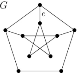
A 1-tough graph is always 2-connected, however, a minimally 1-tough graph is not necessarily minimally 2-connected (see Figure 1), so Mader’s theorem cannot be applied.
G e
Figure 1: A minimally 1-tough but not minimally 2-connected graph. The graph G−e is still 2-connected.
A natural approach to Kriesell’s conjecture is to prove upper bounds on δ(G) for minimally 1-tough graphs. Kriesell’s conjecture states that δ(G)≤2, and the best known upper bound follows easily from Dirac’s theo- rem, yieldingδ(G)≤n/2. Our main result is an improvement on the current upper bound by a constant factor.
Theorem 1.7. Every minimally 1-tough graph has a vertex of degree at most
n 3 + 1.
Toughness is related to the existence of Hamiltonian cycles. If a graph contains a Hamiltonian cycle, then it is necessarily 1-tough. The converse is not true, a well-known counterexample is the Petersen graph. It is easy to see that every minimally 1-tough, Hamiltonian graph is a cycle, since after deleting an edge that is not contained by the Hamiltonian cycle, the resulting graph is still 1-tough.
Let us introduce a class of graphs that is frequently studied while dealing with problems related to Hamiltonian cycles.
Definition 1.8. The graphK1,3 is called a claw. A graph is said to be claw- free, if it does not contain a claw as an induced subgraph.
Problems about connectivity in claw-free graphs can be handled more easily, since every vertex of a cutset is adjacent to at most two components.
We give a complete characterization of minimally 1-tough, claw-free graphs.
Theorem 1.9. If G is a minimally 1-tough, claw-free graph of order n≥4, then G=Cn.
Thus we see that Kriesell’s conjecture is true in a very strong sense if the graph is claw-free. Or equivalently, the family of minimally 1-tough, claw- free graphs is small. On the other hand, we show that in general the class of minimally 1-tough graphs is large.
Theorem 1.10. For every positive rational number t, any graph can be em- bedded as an induced subgraph into a minimally t-tough graph.
The paper is organized as follows. In Section 2 we prove Theorem 1.7 which is the main result of this paper. In Section 3 we prove Theorem 1.9 and in Section 4 we prove Theorem 1.10.
2 Proof of the main result
Here we prove that every minimally 1-tough graph has a vertex of degree at most n3 + 1. First we need a claim that has a key role in the proofs, then we continue with two lemmas.
Claim 2.1. IfG is a minimally1-tough graph, then for every edgee ∈E(G) there exists a vertex set S =S(e)⊆V(G) with
ω(G−S) =|S| and ω (G−e)−S
=|S|+ 1.
Proof. Let e be an arbitrary edge of G. Since G is minimally 1-tough, τ(G−e)<1, so there exists a cutset S=S(e)⊆V(G−e) =V(G)inG−e satisfying that ω (G−e)−S
> |S|. On the other hand, τ(G) = 1, so ω(G− S) ≤ |S|. This is only possible if e connects two components of (G−e)−S, which meansω (G−e)−S
=|S|+ 1and ω(G−S) =|S|. Definition 2.2. LetGbe a minimally 1-tough graph, andean arbitrary edge of G. Let us define k(e) to be the minimal size of the vertex set S guaranteed by Claim 2.1.
In the proof of the next Lemma, we need the following theorem.
Theorem 2.3 ([4]). LetG be a2-connected graph on n vertices withδ(G)≥ n+κ(G)
/3. Then G is Hamiltonian.
Lemma 2.4. LetG be a minimally 1-tough graph on n vertices with δ(G)>
n
3 + 1. Then k(e)> n3 for any e∈E(G).
Proof. Let e be an arbitrary edge ofG. By Claim 2.1 there exists a number k = k(e) and a set of k vertices, whose removal from G−e leaves exactly k+ 1 connected components. Clearly, there is no edge between two different components except e. Among these components there must be one with at mostn−k
k+1
vertices, and inside this component every vertex can have at most n−k
k+1
−1 neighbors. If this component has size 1, then the vertex inside it has degree at most k+ 1 inG, so
n
3 + 1 < δ(G)≤k+ 1,
which means thatk > n3. Otherwise there exists a vertex in this component, which is not an endpoint of e, so its degree in G is at most
n−k k+ 1
−1 +k≤ n−k
k+ 1 −1 +k = n+k2−k−1 k+ 1 . Consider the function
fn(k) = n+k2−k−1 k+ 1 .
Note that for any fixedn,f is monotone decreasing inkif0≤k ≤√
n+ 1−1 and monotone increasing if √
n+ 1−1< k≤n−1.
We show that if k≤ n3, thenδ(G)≤ n3 + 1.
Case 1: 2 ≤ k ≤ n3. Since fn(k) is an upper bound of the minimum degree, it is enough to show that fn(k) ≤ n3 + 1. The above mentioned property of the function implies that it is enough to show this for k = 2 and k = n3.
fn(2) = n+ 1 3 < n
3 + 1, fn
n 3
= n2 + 6n−9
3n+ 9 = (n+ 3)2−18
3(n+ 3) < n+ 3 3 = n
3 + 1.
Case 2: k = 1. Since G is 1-tough, κ(G) ≥ 2. Let e = uv be such an edge, for whichk(e) = 1. Then there exists a single vertexwthat disconnects the graph G− e, so {u, w} or {v, w} is a cutset in G. Thus κ(G) = 2.
Since δ(G)> n3 + 1, by Theorem 2.3 G is Hamiltonian, but G 6=Cn, which contradicts the fact that Gis minimally 1-tough.
Let us define the open neighborhood an edge f = {a, b}. It is the set of vertices adjacent to either a or b excluding a and b.
Lemma 2.5. If G is a minimally 1-tough graph with δ(G) > n3 + 1, then there are two vertices a, b∈ V(G) connected by an edge f ∈ E(G) such that their open neighborhood has size more than 2n3 −1.
Proof. Lemma 2.4 implies that k(e) > n3 for all e ∈ E(G). Let us fix an arbitrary edge e ∈ E(G), and we define x := k − n3. It is easy to see that 0 < x < n6, because removing at least n2 vertices does not leave enough components. Let B :=S(e) denote the set of the removed vertices and let A denote the set of the remaining vertices. Then |A|= 2n3 −x, |B|= n3 +x and by the choice of B the number of components in G−B is also n3 +x.
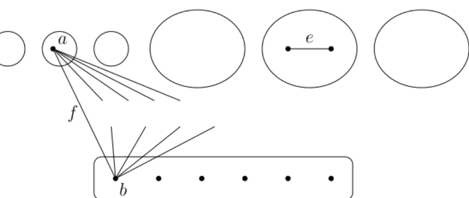
Our strategy is to prove that there exists a vertex b ∈B having at least
n
3 + 1 neighbors in A and among these neighbors there exists a vertex a contained by a component of size at most 2 after the removal of B, see Figure 2. Sincea has more than n3−1neighbors inB\ {b}andb has at least
n
3 neighbors inA\ {a}, their open neighborhood has size more than n
3 −1 + n 3 = 2n
3 −1.
b a
f
e
Figure 2: Finding an edge f for which G−f is 1-tough.
Suppose to the contrary that there exist no such vertices a and b. Let e(A, B) denote the number of edges between A and B. We give a lower and an upper bound for e(A, B), then we show that the lower bound is greater than the upper bound, which leads us to a contradiction.
I. Lower bound: e(A, B)> n92 + n3 +nx+x−4x2.
It is well-known, that the number of the edges in a graph with n0
vertices andk0 components is at most n0−k20+1
. Hence the number of the edges in A is at most
2n
3 −x
− n3 +x + 1 2
= n
3 −2x+ 1 2
.
Since every degree is more than n3 + 1, the following lower bound can be given for e(A, B).
2n 3 −x
n 3 + 1
−2· n
3 −2x+ 1 2
=
= 2n
3 −x n
3 + 1
−n
3 −2x+ 1 n
3 −2x
=
= n2 9 +n
3 +nx+x−4x2 II. Upper bound: e(A, B)< n3 n3 + 1
+x n2 −3x .
To prove the upper bound, we need the following claim.
Claim 2.6. After the removal of B there are at least n6 + 2x
compo- nents of size at most 2.
Proof. After the removal ofB the remaining graph has 2n3 −xvertices and n3 +xcomponents. In every component there must be at least one vertex, so the other 2n3 −x
− n3 +x
vertices can create at most 1
2
2n 3 −x
−n
3 +x
= 1 2·n
3 −2x
= n 6 −x components with size at least 3. So there must be at least
n 3 +x
−n 6 −x
= n 6 + 2x components having size at most 2.
Now we return to the proof of the upper bound. After removing B, the components of size at most 2 have more than n3 neighbors in B. By our assumption, each of these neighbors is connected to less than n3+ 1 vertices in A. Then all the remaining less thanxvertices inB are such that their neighbors in A lie in a component of size at least 3. So all these remaining less than xvertices in B can be adjacent to at most
2n 3 −x
−n
6 + 2x
= n 2 −3x vertices in A.
Hence, there are more than n3 vertices in B that have less than n3 + 1 neighbors in A and the remaining less than x vertices in B have at most n2 −3x neighbors in A, see Figure 3.
> n
3 vertices
< n 3 + 1 neighbors in A
< xvertices
≤ n 2 −3x neighbors in A Figure 3: Giving an upper bound fore(A, B).
Now we show that n2−3x > n3 + 1. Intuitively this means thate(A, B) is maximal if the components of size at most 2 have as few neighbors as possible. This is an easy corollary of the following claim.
Claim 2.7. For the vertices of B, the average number of neighbors in A is more than n3 + 1.
Proof. It is already proved that the number of the edges between A and B is more than
n2 9 + n
3 +nx+x−4x2. We need to show that
n2 9 +n
3 +nx+x−4x2 >|B|n 3 + 1
=n
3 +x n 3 + 1
. Transforming it into equivalent forms, we can see that this inequality holds.
n2 9 +n
3 +nx+x−4x2 > n2 9 +n
3 + n 3x+x 2n
3 x >4x2 n 6 > x
If n2 −3x > n3+ 1did not hold, then each vertex inB could be adjacent to at most n3 + 1 vertices in A, which contradicts Claim 2.7. So the number of the edges between A and B is less than
n 3 ·n
3 + 1
+xn
2 −3x , thus the proof of the upper bound is complete.
Clearly, the lower bound cannot be greater than the upper bound, so n2
9 + n
3 +nx+x−4x2 < n 3 ·n
3 + 1
+xn
2 −3x , 0< x2−n
2 + 1 x, 0< xh
x−n
2 + 1i . This contradicts the fact that 0< x < n6.
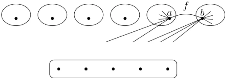
Proof of Theorem 1.7. Suppose to the contrary thatδ(G)> n3+ 1and consider the edgef =abguaranteed by Lemma 2.5. By Claim 2.1 there exist k > n3 vertices, whose removal fromG−f leavesk+1connected components, see Figure 4.
a f b
Figure 4: There are too many neighbors of a and b.
For this we need k+ 1> n3 + 1 independent vertices (one in each of the k+ 1 components), two of them area and b, and the rest of them cannot be adjacent either to a or to b. However, there are less than
n− 2n
3 −1
= n
3 + 1< k+ 1
such vertices, since a and b have more than 2n3 −1 different neighbors. So G−f is 1-tough, which is a contradiction.
3 Claw-free graphs
In this section we prove that minimally 1-tough, claw-free graphs are just cycles (of length at least 4). By the following theorem, the toughness of claw-free graphs can be easily computed.
Theorem 3.1 ([8]). If G is a noncomplete claw-free graph, then 2τ(G) = κ(G).
In our proof we need the following lemmas.
Lemma 3.2. Let G be a claw-free graph with τ(G) = t and S a tough set.
Now the vertices of S have neighbors in exactly two components of G−S, and the components of G−S have exactly 2t neighbors (in S).
Lemma 3.2 follows from the proof of Theorem 3.1, which we do not present here, it can be found as Theorem 10in [8].
Lemma 3.3. If G is a minimally 1-tough graph, then every vertex of any triangle has degree at least 3.
Proof. Suppose to the contrary that {u, v, w}is a triangle and u has degree 2. Let e be the edge connecting v and w. By Claim 2.1 there exists a vertex set S such that ω(G−S) =|S|andω (G−e)−S
=|S|+ 1. Clearly,u∈S and v, w 6∈S. Since the neighbors of u are adjacent, andG is 1-tough
|S|=ω(G−S) =ω G−(S\ {u})
≤ |S| −1, which is a contradiction.
Proof of Theorem 1.9. Suppose to the contrary that Ghas a vertex of degree at least3. Since Gis claw-free, some neighbors of this vertex must be connected, hence there must be a triangle in G. Let us denote the vertices of this triangle by {u, v, w}.
Claim 3.4. For some edge of the triangle{u, v, w}, the vertex set guaranteed by Claim 2.1 has size at least two.
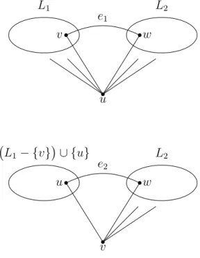
Proof. Suppose to the contrary that for each edge the corresponding vertex set has size 1. Thus for each edge this set must consist of the third vertex of the triangle, i.e. for the edges e1 =vw, e2 =uw and e3 =uv, these sets are S1 :=S(e1) ={u}, S2 :=S(e2) = {v}and S3 :=S(e3) ={w}.
LetL1andL2 denote the connected components of(G−e1)−S1containing v, w respectively. Now the components of (G−e2)−S2 must be L2 and
L1 − {v}
∪ {u}, and the components of (G− e3)−S3 must be L1 and L2 − {w}
∪ {u}. So u cannot have any neighbors in L2 − {w} and in L1− {v}, see Figure 5. This means thatu has only two neighbors v and w, which is a contradiction by Lemma 3.3.
u
L1 L2
v w
e1
v L1− {v}
∪ {u} L2
u w
e2
Figure 5: The vertex u cannot have any neighbors in L2 − {w}.
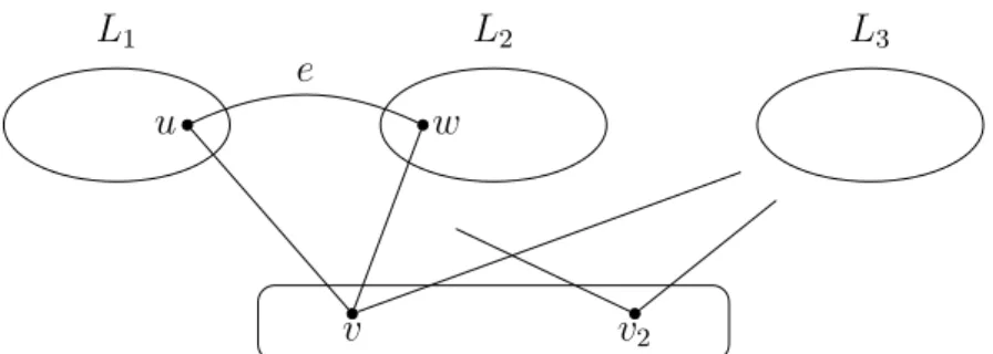
By Claim 3.4 we can assume that for the edge e = uw, the vertex set S =S(e)garanteed by Claim 2.1 has size at least 2. This means that S is a cutset. Since ω(G) =|S|,S is a tough set. So by Lemma 3.2 the component of G−S that contains the edge e has exactly two neighbors in S. One such neighbor must bev, and let us denote the other neighbor byv2. Observe that the set {v, v2} is a tough set. Let L1, L2 denote the connected components of (G−e)− {v, v2} containing u, w respectively and let L3 denote the third connected component, see Figure 6.
v v2
L1 L2 L3
u w
e
Figure 6: The tough set {v, v2} and the setsL1, L2, L3.
Case 1: bothL1 and L2 have size at least 2.
Now {v, v2, u} is a tough set. Using Lemma 3.2 we can conclude that v2
has no neighbors inL2 (since v andu have neighbors inL2), sov2 must have neighbors in L1− {u}, see Figure 7. Using the same argument for the tough set {v, v2, w}, we can conclude thatv2 has neighbors inL2−{w}. Then there is a claw in the graph (it is formed by v2 and one of its neighbors in each of the components L1 − {u}, L2− {w} and L3), which is a contradiction. So we can assume that L1 ={u}.
u v v2
L1− {u} L2 L3
w e
Figure 7: If |L1|>1.
Case 2: L2 has size at least 2 (and L1 ={u}).
Now {v, v2, w} is a tough set, so by Lemma 3.2 v2 is not adjacent to u, so u is a vertex of degree 2, which contradicts Lemma 3.3.
Case 3: L2 ={w}(and L1 ={u}).
By Lemma 3.3, N(u) = {w, v, v2} and N(w) = {u, v, v2}. Consider the edge f = uv and let S′ := S(f) be a vertex set garanteed by Claim 2.1.
Clearly, w ∈ S′, and by Lemma 3.2 w has neighbors in exactly two com- ponents of G −S′. By the choice of S′, the vertices u and v are in the
same component in G−S′, so v2 must be in a different component, which contradicts the fact that uand v2 are adjacent.
4 Embedding graphs into a minimally t-tough graph
In this section we show that for every positive rational number t, any graph can be embedded as an induced subgraph into a minimally t-tough graph.
Our proof is constructive. Different constructions are used for t ≥ 1 and t < 1. For this we need a definition and the following well-known exercises from [6].
Definition 4.1. A graph G is called α-critical, if α(G−e) > α(G) for all e∈E(G).
Lemma 4.2 (Problem 13 of §8 in [6]). Every graph can be embedded as an induced subgraph into an α-critical graph.
Lemma 4.3 (Problem 14of §8 in [6]). If we replace a vertex of an α-critical graph with a clique, and connect every neighbor of the original vertex with every vertex in the clique, then the resulting graph is still α-critical.
Now we proceed with the proof of the case t≥1.
Theorem 4.4. For every positive rational number t ≥ 1, any graph G can be embedded as an induced subgraph into a minimally t-tough graph.
Proof. Let n denote the number of vertices in G and let a, b ∈ N be such that t = a/b. By Lemma 4.2 it is enough to consider the case where G is α-critical. By Lemma 4.3 we can also assume thatb divides n.
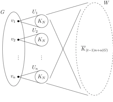
Our strategy is to embed G as an induced subgraph into a graph H, which is not necessarily minimally t-tough yet, but has the following two properties: τ(H) = t and deleting any edge of the induced subgraph of H that is isomorphic to G, lowers the toughness of H. Then if we repeatedly remove an edge from H that does not lower the toughness, the remaining graph will be minimally t-tough (since no further edges can be removed), and the edges corresponding to the subgraph Gare left intact. We define H as follows. Let N be a large integer to be specified later. Let
V :={v1, . . . , vn}, W :={w1, . . . , w(t−1)n+α(G)}
and for each i∈[n] let
Ui :={ui,1, . . . , ui,N}. Then let
U :=
n
[
i=1
Ui
and
V(H) :=V ∪U∪W.
Place the graph G on the vertices of V. For all i ∈ [n] place a clique on Ui
and connect every vertex of Ui to every vertex of W and also to the vertex vi. Note that α(H) does not depend on N, so let us choose N such that N > tα(H). Also note that (t−1)n+α(G) is an integer since b divides n.
See Figure 8.
G v1
v2
...
vn
... KN
KN
KN
U1
U2
Un
W
K(t−1)n+α(G)
Figure 8: The graph H.
Claim 4.5. For each edge e∈E(G), τ(H−e)< t.
Proof. Since G is α-critical, there is an independent set in H −e of size α(G) + 1 among the vertices ofV. Let us delete W and all the vertices of G except this independent set. We deleted
n− α(G) + 1
+ (t−1)n+α(G) =tn−1
vertices from H −e and the resulting graph has n connected components, thus H−e is not t-tough.
Claim 4.6. τ(H)≥t.
Proof. Suppose to the contrary that there exists a cutset X ⊆ V(H) such that ω(H −X) > |X|/t and |X| is minimal. For any i ∈ [n], Ui 6⊆ X, otherwise
α(H)< N
t ≤ |X|
t < ω(H−X)≤α(H),
which is a contradiction. Since X is minimal, we can assume that for any i ∈ [n], Ui ∩ X = ∅, since removing only a proper subset of Ui does not disconnect anything from the graph. Thus W ⊆ X, otherwise H −X is still connected. Let us denote the number of vertices of V ∩X by y. The independence number of the subgraph of H spanned by V ∪U is clearly n, thus ω(H−X)≤n. Which yields
y+ (t−1)n+α(G)
t = |X|
t < ω(H−X)≤n, so
y+α(G)< n.
On the other hand, there are at mostα(G)components ofω(H−X)that contain a vertex of V, the other connected components are some of the Uj, thus ω(H−X)≤y+α(G). Which yields
y+ (t−1)n+α(G)
t = |X|
t < ω(H−X)≤y+α(G), (t−1)n
t <
1− 1
t
y+α(G) , n < y+α(G),
which is a contradiction.
Claim 4.7. τ(H)≤t.
Proof. Let I ⊆ V be an independent set of size α(G) in the subgraph of H induced by V. Let X := (V \I)∪W. Then
|X|=n−α(G) + (t−1)n+α(G) =tn and ω(H−X) =n.
Thus we conclude thatτ(H) =t and the proof is complete.
Remark. A different construction can be obtained as follows. Set N = 1 instead ofN > tα(G), and change the size of W, but connect every vertex of W to every vertex in V, and add a new independent set of verticesW′ which is connected only to W as a complete bipartite graph. The fact that we can assume that Gis α-critical and isolated vertex free, and the appropriate choice of the sizes of W and W′ gives an other good construction. For more details see the alternate proof of Theorem 1.1 in [2].
Note that the construction in Theorem 4.4 cannot be applied for t < 1 since in general (t−1)n−α(G)could be negative. A more interesting reason why this construction does not work in the case t < 1 is that it does not reward us with enough components after deleting a vertex. Thus the core idea of the case t <1is that we introduce multiple Ui for each vertex inV. Theorem 4.8. For every positive rational number t < 1, any graph G can be embedded as an induced subgraph into a minimally t-tough graph.
Proof. Let n denote the number of vertices in G and let a, b ∈ N be such that t=a/b. Similarly to Theorem 4.4, we can assume that G isα-critical.
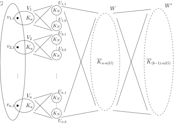
We will embed G as an induced subgraph into H such that τ(H) = a/b, and τ(H−e)< a/b for every edgee of G. The construction is similar as in Theorem 4.4, the same letters denote similar vertices. Let H be defined as follows. Let N be a large integer to be specified later. For each i ∈[n] and j ∈[b], let
Vi :={vi,1, vi,2, . . . , vi,a}, V :=
n
[
i=1
Vi,
Ui,j :={ui,1, . . . , ui,N}, U :=
b
[
j=1 n
[
i=1
Ui,j, W :={w1, . . . , wa·α(G)}, W′ :={w1′, . . . , w(b′ −1)·α(G)},
V(H) :=V ∪U∪W ∪W′.
Place the graph G on the vertices v1,1, . . . , vn,1 and for each i ∈ [n] place a clique on Vi. For each i ∈ [n], j ∈ [b] put a clique on Ui,j and connect every vertex in Ui,j to every vertex in W and Vi. Connect every vertex in W to every vertex in W′. Observe that α(H) does not depend on N, so let N > tα(H). See Figure 9.
G v1,1
v2,1
...
vn,1
V1
V2
Vn
Ka
Ka
Ka
...
...
...
... KN
KN
KN
KN
KN
KN U1,1
U1,b
U2,1
U2,b
Un,1
Un,b
W W′
Ka·α(G) K(b−1)·α(G)
Figure 9: The graph H.
Claim 4.9. For each edge e∈E(G), τ(H−e)< a/b.
Proof. By the α-criticality of G, the graph G−e has an independent set I ⊆ V(G) of size α(G) + 1. Let us delete the vertices of W and for every i∈[n], if vi ∈/ I then let us also delete Vi. We deleted exactly
n−(α(G) + 1)
a+α(G)·a = (n−1)a
vertices. After the deletion, the vertices of I are in different connected com- ponents and the vertices of W′ are isolated. There are n −(α(G) + 1)
b more connected components not containing any vertex fromGbut containing vertices from U. Thus the resulting graph has
α(G) + 1
+ (b−1)·α(G) + n−(α(G) + 1)
b= (n−1)b+ 1 connected components which is one more than an a/b-tough graph could have.
Claim 4.10. τ(H)≥a/b.
Proof. Suppose to the contrary that there exists a set of vertices X⊆V(H) such thatω(H−X)>|X|/t. First we show that some convenient assumptions can be made for X.
Lemma 4.11. We can assume that X has the following properties.
(1) If some vertices have the same closed (or open) neighborhood, then either all or none of them are in X.
(2) For every i∈[n] and j ∈[b], Ui,j∩X =∅. (3) W ⊆X.
(4) For all i∈[n], either Vi ⊆X or Vi∩X =∅. (5) W′∩X =∅.
Proof.
(1) Removing only a proper subset of such a vertex set does not disconnect anything from the graph.
(2) Since for alli∈[n]andj ∈[b]the closed neighborhoods of the vertices of Ui,j are identical, by (1) eitherUi,j ⊆X orUi,j∩X =∅. But by the choice of N, Ui,j 6⊆X, otherwise
α(H)≤ N
t ≤ |X|
t < ω(H−X)≤α(H), which is a contradiction.
(3) Otherwise by (2) H−X would be connected.
(4) For all i∈[n], the closed neighborhood of vi,1 is larger than the closed neighborhood of the vertices vi,2, . . . , vi,n, so if vi,1 6∈ X, then we can assume thatVi∩X =∅. If vi,1 ∈X, then we can assume thatVi ⊆X, since adding the rest of Vi to X would increase the size of X by at most a−1 and the number of the components by exactly b−1. This preserves the property thatω(H−X)>|X|/t, as a < b.
(5) It is a trivial consequence of (3).
Let y be the number of the sets Vi that are subsets of X. There are at most α(G) components of H −X that contain a vertex from V, the other connected components are some of the components of U and every vertex of W′. Thus ω(H−X)≤α(G) +by+ (b−1)·α(G). By our assumption that
|X|/t < ω(H−X) this yields ay+aα(G)
t = |X|
t < ω(H−X)≤α(G) +by+ (b−1)·α(G).
Since t=a/b,
b ay +aα(G)
< a by+bα(G) , which is a contradiction.
Claim 4.12. τ(H)≤a/b.
Proof. Let I ⊆ V(G) = {v1,1, . . . , vn,1} be any independent set of size α(G) and consider the set
X =[
{Vi| v1,i ∈/ I}
∪W. Since
|X|=a n−α(G)
+aα(G) =an and H−X has exactly
α(G) +b n−α(G)
+ (b−1)·α(G) =bn connected components.
So τ(H) =a/b and the proof is complete.
Acknowledgement
We thank the anonymous reviewers for their careful reading of our manuscript and their many insightful comments and suggestions. All authors are par- tially supported by the grant of the National Research, Development and Innovation Office – NKFIH, No. 108947. The first author is also supported by the National Research, Development and Innovation Office – NKFIH, No. 116769. The second author is also supported by the National Research, Development and Innovation Office – NKFIH, No. 120706.
References
[1] D. Bauer, H. J. Broersma, and H. J. Veldman,Not every 2-tough graph is Hamiltonian, Discrete Applied Mathematics 99(2000), 317–321.
[2] D. Bauer, A. Morgana, and E. Schmeichel, On the complexity of recognizing tough graphs, Discrete Mathematics124(1994), 13–17.
[3] V. Chvátal, Tough graphs and hamiltonian circuits, Discrete Mathematics 5 (1973), 215–228.
[4] R. Häggkvist and G. G. Nicoghossian, A remark on Hamiltonian cycles, Journal of Combinatorial Theory, Series B 30(1981), 118–120.
[5] T. Kaiser, Problems from the workshop on dominating cycles, http: // iti. zcu. cz/ history/ 2003/ Hajek/ problems/ hajek-problems. ps. [6] L. Lovász,Combinatorial problems and exercises, AMS Chelsea Publishing, Providence,
Rhode Island, 2007.
[7] W. Mader, Eine Eigenschaft der Atome endlicher Graphen, Archiv der Mathematik 22 (1971), 333–336.
[8] M. M. Matthews and D. P. Sumner, Hamiltonian results inK1,3-free graphs, Journal of Graph Theory8(1984), 139–146.