RELATIVE EFFECTIVENESS OF THE TRUST-REGION ALGORITHM WITH PRECISE SECOND ORDER
DERIVATIVES
Ambrus K ˝oházi-Kis∗
Department of Natural Sciences and Engineering Basics, GAMF Faculty of Engineering an Computer Science, John von Neumann University, Hungary
Keywords:
Levenberg-Marquardt–method Trust-region method
Hessian matrix Eigen-value problem Numerical stability Article history:
Received 7 September 2018 Revised 2 April 2019
Accepted 19 March 2019
Abstract
Trust-region methods with precise Hessian matrix have some drawbacks: time consuming calculation of the elements of the second order derivative matrix, and the generally non-definite Hessian matrix causes numerical and methodical troubles. Their applicability depends on how well their substitute, for example the Levenberg-Marquardt–method performs. The Levenberg- Marquardt–method often performs well in least-squares prob- lems. This procedure dynamically mixes the steepest-descent and the Gauss-Newton–methods. Generally one hopes that the more analytical properties of the problem’s cost function utilized in an optimization procedure, the faster, the more effective search method can be constructed. It is definitely the case when we use first derivatives together with function values (instead of just func- tion values). In the case of second derivative of the cost function the situation is not so clear. In lot of cases even if second order model is used within the search procedure the Hessian matrix is just approximated, and it is not calculated precisely even if it would be possible to calculate analytically, because of its tem- poral cost and a big amout of memory needed. In this paper I investigate whether the precise Hessian matrix is worth to be determined, whether one gains more on the increased effective- ness of the search method than looses on the increased tempo- ral costof dealing with the precise Hessian matrix. In this paper it is done by the comparison of the Levenberg-Marquardt–method and a trust-region method using precise Hessian matrix.
1 Introduction
Least-squares problems are quite frequent in numerical data processing [1, 3].
Let us take a function f : Rn 7→Rm (withm > n), called asresidual vector, and consider the problem of finding the least-squares solutionx†
x†=ArgM in{F(x)} , (1)
where functionF : Rn7→Ris called thecost function(orfunction of merit) of the problem:
F(x)≡ 12
m
X
i=0
(fi(x))2 . (2)
∗Corresponding author. Tel.: +3676516436; fax: +3676516299 E-mail address: kohazi-kis.ambrus@uni-neumann.hu
1
When the components fi(x) off(x) are non-linear functions, we have to use iteration: from a starting pointx0we computex1,x2,x3, ...and we shall assume that the descending condition
F(xk+1)< F(xk) (3)
is satisfied.
The solution gets much faster, if the derivatives of the cost function can be determined. In this paper only this kind of least-squares problems are considered.
The derivative function of anmvariable,ndimensional vector-functionf : Rn 7→Rmis also called Jacobian-matrix (see Ref. [4] ):
f0(xi)≡ df dx x=x
i
=Jf(xi)≡
∂ f1
∂ x1
x=xi
· · · ∂ x∂ f1
n
x=xi
... . ...
∂ fm
∂ x1
x=xi
· · · ∂ f∂ xm
n
x=xi
. (4)
The first derivative of the functionF(x)≡ 12 kf(x)k2 can be obtained as (see ref. [1])
F0(xi) =Jf(xi)T f(xi) (5)
F0(xi)≡
∂ F
∂ x1
x=xi
...
∂ F
∂ xn
x=xi
=
∂ f1
∂ x1
x=xi
· · · ∂ f∂ xm
1
x=xi
... . ...
∂ f1
∂ xn
x=xi
· · · ∂ f∂ xm
n
x=xi
f1(xi) ... fm(xi)
. (6)
The second derivative of functionF, the Hessian-matrix can be calculated as (see ref. [1]) F” (xi) =Jf(xi)T Jf(xi) +f” (xi) f(xi) . (7) There are strategies that use the derivatives of the cost function to solve optimization problems [1]. A short survey is given among the fundamental methods to give some insight to the connection between the Levenberg-Marquardt–algorithm and trust-region methods.
In the following I investigate the possibility to gain effectiveness when we use trust-region algo- rithm in which the precise Hessian matrix of the cost function is determined instead of the Levenberg- Marquardt–algorithm in which the Hessian matrix is just approximated.
2 Fundamental methods
2.1 Steepest descent direction method Ahdescent direction satisfies
hT F0<0., (8)
In the steepest descent direction method linear search is proceed though a direction
hsd=−F0 . (9)
The method is robust even if xis far from x†, but it has poor convergence. Especially the low speed of final convergence is problematic.
2.2 Newton’s method
Second order expansion of the residual vector is used to calculate the second derivative of the cost function
F(x+ξ)'F(x) +ξT F0(x) +12ξT F” (x) ξ+O kξk3
, (10)
F0(x+ξ)'F0(x) +F” (x)ξ. (11)
The optimization stephis the solution of the equation,
F” (x) hN =−F0(x) . (12)
Newton method performs well in the final stage of the iteration, where x ' x? and the Hes- sian matrix is positive definite, we get quadratic convergence. In the opposite situation, i.e. when the Hessian matrix is negative definite or indefinite, generally one cannot get even a descent step when one uses equation 12. If the eigenvalues and eigenvectors of the Hessian are determined the Newton’s-method can be made an effective tool even if the Hessian is not positive definite [2].
2.3 Gauss-Newton method
This method is also called quasi-newton method because the Hessian matrix is approximated, the second term of the Hessian is omitted in (7):
F” (xi)'Jf(xi)T Jf(xi) . (13) The optimization step is the solution to
Jf(xi)T Jf(xi)hN G =−F0(xi) (14) The obtained directionhN G is always descent [1] if he Jacobi-matrixJf(x)has full rank.
The approximation is good, the convergence is quadratic if f(xi) is small enough, or f” (xi) is negligible (quasi-linear least square problem).
The value ofF x†
controls the final convergence speed.
The method with line search can be shown to have guaranteed convergence, provided that {x|F(x)≤F(x0)}is bounded, and the Jacobian-matrixJf(x)has full rank in all steps [1].
If the applied approximation for the second derivative of the cost function is not good, the conver- gence is generally slow.
3 Levenberg-Marquardt method
Levenberg (1944) and Marquardt (1963) suggested a method where the step his computed by the following equation:
h
Jf(xi)T Jf(xi) +µI i
h=−F0(xi) , F0(xi) =Jf(xi)T f (15) whereI is the unity matrix, and µ >0is the so called damping parameter. This parameter controls the size and also the type of the step. For allµ >0the coefficient matrix is positive definite, and this ensures thathis a descent direction.
This method is a combination of the Gauss-Newton method and the steepest-decent method [1, 4, 5]. For large values ofµwe get
h' −1
µF0(xi) , (16)
i.e. a short step in the steepest-descent direction.
If µ, however, is very small, then h = hN G, which is a very good step in the final stages of the iteration (whenxiis close tox†, the solution) if the residual valuef x†
is small enough.
The method is self-controlled by the gain factor
ρ= F(x)−F(x+h)
L(0)−L(h) , (17)
where the denominator is the gain, predicted by the linear model:
L(h) =F(xi) +hT F0(xi) +12hTJf(xi)T Jf(xi)h (18) L(0)−L(h) = 12hT
µh−F0(xi)
>0 (19)
Ifρis large thenL(h)is a good approximation toF(x+h), we can decreaseµthat the next step should be closer to the Gauss-Newton step. If ρ is small but positive thenh is a descent step but µmust be increased, that the next step should be closer to the steepest-direction step because the second order approximation ofF(x+h) is not good enough. Ifρ is negative then h is not even a descent step, the step must be canceled,µmust be increased, that the next step should be closer to the steepest-direction step because the second order approximation ofF(x+h)is not good enough.
4 Trust-region methods
A trust-region optimization method defines a region (with its radius) around a test point. Within this region a simplified (usually not more than second order) model is built. The optimization step is determined by the optimal point of the model function within this region where the model function is trusted to be a good model of the cost function. [1]. If the improvement is well modelled by the model function than the step is executed and the radius of the trust region may be increased, otherwise the step is cancelled and the radius is decreased.
The earliest use of the term seems to be by Sorensen in 1982 [6].
There exist also trust-region methods without derivatives [7] that form a linear or quadratic models by interpolation to values of the cost function.
There are trust-region methods that uses only the first derivative of the residual vectorf. A classic method of this kind is the Powell’s dog-leg method [10]: it combines the steepest-descent (hsd) and the Gauss-Newton (hGN) steps to get a step (hdl) not longer than the sugar (R) of the trust-region.
In some sense Levenberg-Marqhardt method is also a trust region method: by controlling the damping parameterµthe step length is controlled.
In the case of the true second order derivative Hessian matrix, the trust-region step can be calcu- lated only if the eigenvalues and eigenvectors of the Hessian is determined [2]. Without solving the eigen-problem of the Hessian the trust region step can be calculated only iteratively [8, 9].
In the following I will concentrate on second order trust-region methods that build a true second order model of the cost function.
4.1 Second-order trust-region methods
These kind of trust-region methods are based on the second order model of the merit function obtained from the Taylor-expansion off,
F(xi+ξ)'L(ξ) =F(xi)−ξTb+12ξT H ξ, (20) where the derivatives of the cost functionF(xi)are exactly calculated
b=−Jf(xi)T f , H =Jf(xi)T Jf(xi) +f” (xi) f(xi) . (21) A constrained optimization is made in the trust-region to find the minimizer of the model function.
The subspace optimization can be done inexactly but in this way the benefit of using the exact Hessian matrix is (partly) wasted.
Exact subspace optimization even of the model function can be very time-consuming because of the need for solving of the eigen-problem of the Hessian-matrix. However, when the calculation of the cost function is quite time consuming then the extra time of the evaluation of the eigen-problem of the Hessian can be negligible.
4.2 Path-finder trust-region algorithm
I proposed a trust-region method that is easy to implement: instead of searching for an optimal value, the optimal way to the minimizer of the original problem is followed within the trust region [11].
It can be supposed that the way along the local gradient to the local minimizer can be parametrized with some scalar (time-like) parametert. The path towards the minimizer of the model function can be determined, as long as the eigen-system of the symmetric Hessian matrix H is found. The eigen-vectors and eigen-values can be effectively determined with thetred2 andtqli functions of the Numerical Recipes [12]. Thetred2andtqli functions work well up to 100 dimensions when one uses long doublereal variable in C.
The way toward the minimizer leads anti-parallel to the local gradient:
dx
dt =b−H x. (22)
This equation is separated in the eigen-system ofH dxj
dt =bj−λjxj, (23)
where xj and gj are the j-th component of the vectors x and g, respectively; and λj is the j-th diagonal element ofH in its eigen-system of coordinate. This equation can be integrated. Ifλj 6= 0 (or more precisely|λj|> ε, whereεis a small number) then
xj(t)−xi j= bj
λj [1−exp (−λjt)] , (24)
wherexi is the starting point. Otherwise (ifλj ≈0) (or more precisely|λj| ≤ε)
xj(t)−xi j =bjt . (25)
The region can be trusted only within an environment of radiusR, that is the length of our step r(t) =
m
X
i=1
kx(t)−xik2 (26)
could not be longer than R. Even if the Hessian matrix H is positive definite (all of its eigenvalues are positive) it cannot be longer than R. The restriction of r(t) can be done by a one-dimensional successive approximation int.
Finally one has to check that how good the second order approximation was. Depending on the value of the gain factorρin Eq. (17) one has to increase (ρ > ρ0>0) or decrease (ρ≤ρ0) the radius of our trust region, and one even has to cancel the step ifρ≤0.
5 Comparison the efficiencies of LM and my trust-region method
The Path-finder trust-region algorithm described above is just a true second order method. In the following the Levenberg-Marquardt–method is tested: when it performs worse than a true second- order method.
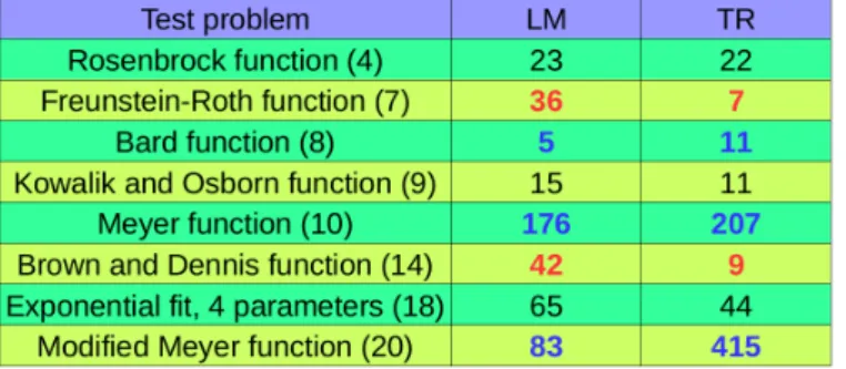
I compared the performances of the Levenberg-Marquardt (LM) and Trust-Region (TR) methods on problems from the Ref. [4].
Table 1. Levenberg-Marquardt (LM) and Trust-Region (TR) methods step numbers to achieve the minimizers of different optimization problems to the same accuracy
It can be seen in table 1. that in some problems the true second order trust-region method performs better. It seems that in these problems the approximations applied in the Levenberg- Marquardt–method are not good enough. In other problems the Levenberg-Marquardt–method per- forms even better than my trust-region method. The most significant case is the Modified Meyer function’s problem where I beleive that the numerical instability of my method emerged in this case is the origin its partial failure. In my trust region much more problematic eigen-problems must be solved than in the case of Levenberg-Marquardt– method where only matrix inversion is made.
It needs additional investigations on different problems why the one or the other method performs better on.
Acknowledgement
This research is supported by EFOP-3.6.1-16-2016-00006 "The development and enhancement of the research potential at John von Neumann University" project. The Project is supported by the Hungarian Government and co-financed by the European Social Fund.
References
[1] J. Nocedal, S.J. Wright, “Numerical Optimization”, Springer-Verlag (1999).
[2] W. Shiquan, W. Fang, “Computation of a trust region step”, Acta Math. Appl. Sinica, 7, 354-362 (1991).
[3] K. Madsen, H.B. Nielsen, O. Tingleff, “Methods for non-linear least square prob- lems”, IMM Department of Mathematical Modeling, Technical Paper, booklet 1999.
(Available: http://www.imm.dtu.dk/pubdb/views/edoc_download.php/ 3215/pdf/imm3215.pdf Ac- cessed: 2018.11.05.)
[4] H.B. Nielsen, “Damping parameter in Marquardt’s method”, IMM Depart- ment of Mathematical Modeling, Technical Paper, booklet 1999. (Available:
http://www2.imm.dtu.dk/documents/ftp/tr99/tr05_99.pdf Accessed: 2018.11.05.)
[5] D. Ramadasan, M. Chevaldonné, T. Chateau, “LMA: A generic and efficient implemen- tation of the Levenberg-Marquardt Algorithm”, Sotfware: Praxtise and Experience, doi:
10.1002/spe.2497 (2017).
[6] D.C. Sorensen: Newton’s Method with a Model Trust Region Modification, SIAM J. Numer. Anal., 19(2), 409426 (1982).
[7] B. Karasözen, “Survey of trust-region derivative free optimization methods”, J. of Industr. and Managm. Optim., 3, 321-334 (2007).
[8] J.B Erway, P.E. Gill, J.D. Griffin, “Iterative methods for finding a trust region step”, SIAM J. Optim., 20, 1110-1131 (2009).
[9] J.B Erway, P.E. Gill, “A subspace minimization method for the trust-region step”, SIAM J. Optim., 20, 1439-1461 (2009).
[10] M.J.D. Powell, “A hybrid method for non-linear Equations”, In P. Rabinowitz (ed): Numerical methods for non-linear algebraic equations, Gordon&Breach, pp. 87-114 (1970).
[11] A. K ˝oházi-Kis, “Dielektrikumtükrök automatizált tervezése”, GAMF Közleményei, XXIII. év- folyam, 87-95 (2009).
[12] W.H. Press, S.A. Teukolsky, A.W.T. Vetterling, A.B. Flannery, Numerical Recipes in C: The Art of Scientific Computing, Cambridge University Press, New York, 1992.