Stabilization and destabilization of the equilibria of the pendulum
Outline of PhD Thesis
LÁSZLÓ CSIZMADIA
SUPERVISOR:
DR. LÁSZLÓ HATVANI PROFESSOR EMERITUS
DOCTORAL SCHOOL OF MATHEMATICS AND COMPUTER SCIENCE UNIVERSITY OF SZEGED
FACULTY OF SCIENCE AND INFORMATICS BOLYAI INSTITUTE
SZEGED 2018
1 Introduction
In the thesis we investigate motions of an excited pendulum about their equilib- ria. The excitation means a step-function coefficient in the equation of motion, namely in a second order linear eqaution which describes the motions around the upper and the lower equilibrium states. We are looking for the values of the parameters in the excitation for which the upper equilibrium is stable, and the lower one is unstable. Our method is elementary in the sense that instead of dif- ficult calculations of the Floquet Theory - the classical theory of the differential equation with periodic coefficient - simply geometric ideas are applied.
After a short foreword and introduction, we investigate the problem of swing- ing. Introducing the concepts of solutions going away from the origin and ap- proaching to the origin, we give necessary and sufficient conditions in terms of T andεfor the existence of solutions of these types, which yield conditions for the existence of periodic solutions of the equation of motion.
In the next chapter, we study the stability of the upper equilibrium of the pendulum. An earlier published method ([28]) is improved to the arbitrary inverted pendulum and thanks to this we give a sharper estimate for the stabi- lizability of the upper equilibrium.
Finally, we investigate the stability of the upper equilibrium, again. The equation of motion of the pendulum around the upper equilibrium is a differ- ential equation with a 2T-periodic step function coefficient. We construct the 2T- and the 4T-periodic solutions of this equation. The curves on the param- eter plane corresponding to the 2T- and the4T-periodic solutions describe the boundaries of the stability zone, so we can specify the exact stability map.
The dissertation is based on the following papers of the author:
• L. Csizmadia, L. Hatvani, An extension of the Levi-Weckesser method to the stabilization of the inverted pendulum under gravity, Meccanica, 49(2014), 1091–1100.
• L. Csizmadia, L. Hatvani, On a linear model of swinging with a periodic step function coefficient,Acta Sci. Math. (Szeged),81(2015), 483–502.
• L. Csizmadia, L. Hatvani, On the existence of periodic motions of the excited inverted pendulum by elementary methods (submitted).
In this outline we use the same notations and numberings (apart from the labels of the formulae) as in the thesis.
Preliminaries
The mathematical pendulum is a particle connected by an absolute rigid and weightless rod which length is l = const. [1, 8] One of the state variables is the angle (ψ) between the rod of the pendulum and the direction downward measured counter-clockwise, the other one is its derivative respect to the time.
If the particle is only subjected to gravity, then motions of the mathematical pendulum are described by the second order differential equation
ψ¨+g
l sinψ= 0 (−∞< ψ <∞). (1)
As we can see from equation (1), the system has two equilibrium positions:the lower one (ψ≡0 (mod 2π)) is stable and the upper one (ψ≡π (mod 2π)) is unstable. Stability in the first approximation of nonlinear systems which has been described by Lyapunov [31] means that the original, nonlinear - perturbed - system is approximated by a suitable linear - unperturbed - system. Now, we linearize the equation (1) in the neighbourhoods of the equilibria: U0 ésUπ. If ψ ∈U0 then sinψ≈ψ, and if ψ ∈Uπ thensinψ ≈ −ψ+π=−(ψ−π). Let θ :=ψ−π. So, ifψ =π thenθ = 0. The linear equations of motions around the lower and the upper equilibrium position are
ψ¨+g
lψ= 0, θ¨−g
lθ= 0. (2)
We can rewrite the equations into the form
¨
x±a2(t)x= 0, a(t) :=ak, iftk−1≤t < tk (k∈N),
where {ak}∞k=1,{tk}∞k=0 sequences of positive numbers such thattk < tk+1, for allk∈N, furthermore,limk→∞tk =∞andt0:= 0.
When we want to stabilize the upper equilibrium and destabilize the lower one, the coefficient of equations (2) is not constant: it is a periodic function.
We investigate the cases when the coefficient is a periodic step function and one period has two steps. In [16] the author introduces and in [17] explains a method by which equations (2) can be rewritten into an impulsive dynamical system. Namely, around the lower equilibrium the appropriate system is
˙
x=aky, y˙=−akx (tk−1≤t < tk), x(tk) =x(tk−0), y(tk) = ak
ak+1y(tk−0) (k∈N). (3) The system which describes the motions around the upper equilibrium is
˙
x=aky, y˙=akx (tk−1≤t < tk), x(tk) =x(tk−0), y(tk) = ak
ak+1
y(tk−0) (k∈N), (4)
wheref(t−0)denotes the left-hand side limit of functionf att. The expression
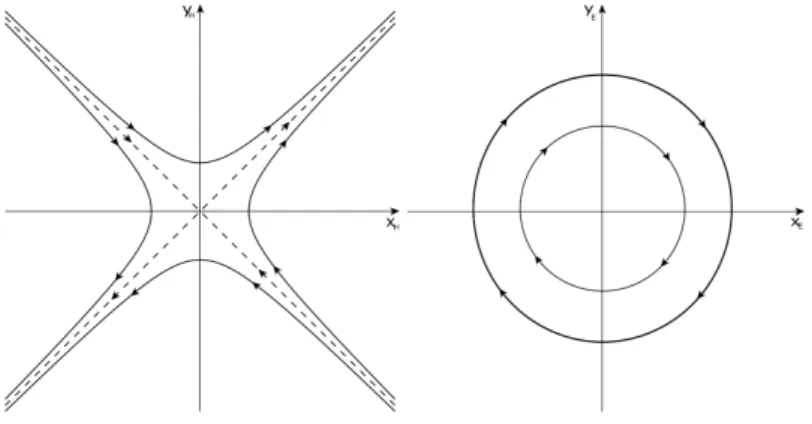
"impulsive" means that between the continuous parts of (3) and (4) there is a vertical contraction/dilation. It is not difficult to show that the continuous components of the dynamics of (3) are uniform clockwise “elliptic (ordinary) rotations" around the origin with the angle velocity ak, and the continuous parts of (4) are “hyperbolic rotations", so the phase point moves on circles around the origin and on hiperbolae, see Figure 1.
Figure 1: Hyperbolic and elliptic rotation
2 On the problem of swinging
A swing, as a physical pendulum is equivalent to a mathematical pendulum of an appropriate length [25], provided that the swinger is motionless. However, the swinger wants to destabilize the pendulum, so he/she moves squatting and raising consecutively. As a result, the distance of the center of gravity of the physical pendulum from the suspension point (i.e, the length of the mathemat- ical pendulum) changes in time periodically [1], and motions are described by the equation
¨
x+a2(t)x= 0,
a(t) :=
a1:=
r g
l−ε, if 2kT ≤t <(2k+ 1)T, a2:=
r g
l+ε, if (2k+ 1)T ≤t <(2k+ 2)T, (k= 0,1, . . .), (5) where xdenotes the angle between the rod of the pendulum and the direction downward measured counter-clockwise;gandl are the gravity acceleration and the length of the rod, respectively;ε >0is a parameter measuring the intensity of swinging,T >0is the half period of the variation of length of the pendulum.
The problem of swinging is to find the instability domain on the parametric plane (T, ε)to the excited equation (5) (problem of parametric resonance), so that subspace where the solutionx= 0of (5) is unstable.
The Floquet-theory is the method of study of linear differential equations with periodic coefficient. It follows from this theory that ifΦ(t)is a fundamental matrix solution of (5) such that Φ(0) = E, where E is 2×2 identity matrix, then if |Tr Φ(T)| < 2, then solution x = 0 of (5) is stable, furthermore, if
|Tr Φ(T)|>2, thenx= 0is unstable.
The calculations based on Floquet-theory often lead to series expansion, difficult numerical computations and estimates. Our aim to give the exact instability domain for the swinging thus we show a more elementary treatment.
But it is important that the boundary of the instability domain is described by the equation |Tr Φ(T)|= 2. We prove by the use of a geometric method that the boundary curves of type T =f(ε), T =g(ε)consist of points of the plane for which (5) has either2T-periodic or4T-periodic solutions, andf(ε),g(ε)go to one of the points((k/2)(πp
l/g),0) (k∈N)asε→0. This result harmonizes with experiences: for small ε >0 (a child wants to swing), period of swinging has to be equal to one of the critical half-periodT = (k/2)(πp
l/g),(k∈N).
As first step, we find conditions guaranteeing that the trajectory t7→(x(t;x0,x˙0),x(t;˙ x0,x˙0))of (5) starting from a pointP(x0,x˙0)of the(x,x)˙ plane returns to a point of the line L through the origin (0,0) and P in the sense that (x(2T;x0,x˙0),x(2T˙ ;x0,x˙0)) ∈ L. Such a solution is either going away from the origin, or approaching to the origin, or periodic of either 2T or 4T. If the two points have the same distance from the origin then the solution is either2T-periodic or4T-periodic. To transform (5) into an equation containing the period of excitation explicitly as a parameter, introduce the so called non- dimensional timeτ = (L/T)t and so we consider the motion of the phase point as the function ofL. The impulsive system (3) can be interpreted by a discrete system on the plane(x, y): introduce the polar coorinates(r, ϕ)by equations
x=rcosϕ, y=rsinϕ (r >0,−∞< ϕ <∞).
Then the equivalent discrete system is xk+1
yk+1
!
=C ak+1
ak+2
R(ak+1(tk+1−tk)) xk yk
!
(k= 0,1,2, . . .), (6) where R(θ) denotes the matrix of rotation and C(κ) denotes the matrix of contraction-dilation. The initial state of the phase point is(r0, ϕ0).
Definition 2.1. A solution of the system (6) corresponding to the model of the swing is called angle-periodic modulo2π (respectively,4π) if
ϕ(2L)≡ϕ0 (mod 2π), respectively, ϕ(2L)≡ϕ0−π (mod 2π).
Definition 2.2. An angle-periodic solution of the system (6) corresponding to the model of the swing modulo 2π or 4π is called approaching (to the origin) (respectively, going away (from the origin)) if
r(2L)< r0, respectively, r(2L)> r0.
Using the concept which has just been introduced, we give a necessary and sufficient condition for the existence the 2T- and 4T-periodic solutions of the equation of motion.
Theorem 2.3. For every ε > 0 there are sequences {Tk(ε)}∞k=1, {Tek(ε)}∞k=1 such that equation(5)withT =Tk(ε)(respectively, withT =Tek(ε)) has2Tk(ε)- periodic (respectively, 4Tek(ε)-periodic) solutions. In addition,
0<Te1≤Te2< T1≤T2<Te3≤Te4< . . .; lim
k→∞Tk =∞, (7)
and
ε→0+0lim 2T2p+1(ε) = lim
ε→0+02T2p+2(ε) = (2p+ 2) 1 2 2π
s l g
!!
,
ε→0+0lim 2Te2p+1(ε) = lim
ε→0+02Te2p+2(ε) = (2p+ 1) 1 2 2π
s l g
!!
hold for all p∈N.
Due to the Theorem 2.3 we can prove the theorem which describes the instability zones.
Theorem 2.4. The inside of the domain of instability (parametric resonance) on the parameter plane(T, ε)for equation (5) is
∪0<ε<l(∪∞p=0({(T, ε) :T2p+1(ε)< T < T2p+2(ε)}
∪ {(T, ε) :Te2p+1(ε)< T <Te2p+2(ε)})) (Tk,Tek were defined in (7)).
3 Stabilization of the upper equilibrium
At the beginning of the last century A. Stephenson has discovered [34, 35]
that the upper (unstable) equilibrium of the mathematical pendulum can be stabilized by vibrating of the point of suspension vertically with sufficiently high frequency. The motions around the upper equilibrium was investigated by P. L. Kapitsa in detail in 1951 [23, 24], and since then this phenomenon is called Kapitsa’s pendulum. M. Levi and W. Weckesser [28] gave a simple geometrical explanation for the stability effect provided that the frequency is so
high that the gravity can be neglected, and the two half-periods of the periodic excitation of the parameter is symmetric. The Levi-Weckesser method does not work in the case when there acts gravitation, so it is a very natural challenge to find an extension of the method to this more natural case. We extend the Levi-Weckesser method to the arbitrary inverted pendulum not assuming even symmetricity between the upward and downward phases in the vibration of the suspension point. We can improve the method and give a sharper estimate for the frequency in the gravity-free case, too.
As in [28], we suppose that the acceleration of the suspension point of the pendulum is
a(t) :=
A,if kT ≤t <(2k+ 1)T 2,
−A,if (2k+ 1)T
2 ≤t <(k+ 1)T, (k= 0,1, . . .).
(8)
So, the functiona(t)isT-periodic. The equation of motion is ψ¨−1
l(g+a(t))ψ= 0. (9)
The authors supposed that A >> gandg= 0in equation (9). Introducing the quantityω=p
A/l, (9) can be written into the form ψ¨±ω2ψ= 0,
where the sign changes corresponding to the functiona(t).
Theorem 3.1 (M. Levi, W. Weckesser; [28]). Consider the inverted pendulum (9) in the gravitation-free case (g = 0) provided that the suspension point is vibrated symmetrically (Ah=Ae=A >>1; consequently,Th=Te=T /2). If
ωT < π ω:=
rA l
!
, (10)
then (9)is strongly stable.
Equation (9) is calledstrongly stableif it is stable and it remains stable under sufficiently small perturbations. There are two different phases corresponding to the values of function a(t) in (8). The two phases mean two different rota- tions on the phase plane, and the authors’ method is based upon the geometrical observation that the superposition of two consecutive rotations has no real eigen- values if it turns every non-zero vector of R2 with a non-zero angle (mod π).
In the present chapter we estimate this angle for an arbitrary vector ofR2. Suppose now that the suspension point is vibrating vertically with the T- periodic acceleration
a(t) :=
Ah ifkT ≤t < kT +Th,
−Ae ifkT+Th≤t <(kT +Th) +Te, (k= 0,1, . . .) ;
(11)
whereAh, Ae, Th, Teare positive constants (Th+Te=T) so that the motion of the suspension point isT-periodic. Indicesh andepoint to the hyperbolic and the elliptic phase of the motion, respectively. The equation of motion is given in the form of (9). We can state the next theorem.
Theorem 3.2. Let Rem(ϕ;π)denote the reminder of the real number ϕ∈R modulo π(0≤Rem(ϕ;π)< π).
If
2 arctaneωhTh−1 eωhTh+ 1 + 4
arctan rωh
ωe
−π 4
<min{Rem(ωeTe;π); π−Rem(ωeTe;π)},
(12)
then equation (9) is strongly stable, where ωh:=
rAh+g
l , ωe:=
rAe−g l .
Due to the differentωh and ωe, between the hyperbolic and elliptic phases two impulsive effects, so called “jumps" happen to the phase point during one period, as we have written in Introduction. Applying Theorem 3.2 to the gravitation-free and symmetric case we get the following extension and approve- ment of Levi’s and Weckesser’s result:
Corollary 3.3. Suppose that g= 0 andAh=Ae=A in (9). If 4 arctaneωT /2−1
eωT /2+ 1 <
<min{Rem(ωT; 2π); 2π−Rem(ωT; 2π)},
(13)
then (9)is strongly stable.
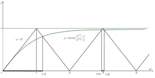
Corollary 3.3 essentially improves Theorem 3.1. In fact, 4 arctaneωT /2−1
eωT /2+ 1 < ωT (0< ωT < π),
so the first stability interval on the ωT-axis satisfying (13) is (0,3.75. . .) (see Figure 2) instead of (0, π)yielded by (10). Besides, Corollary 3.3 also extends Theorem 3.1 finding stability intervals on ωT-axis after2π (see the thickened intervals on Figure 2). This can be interpreted mechanically that stabilization is possible with arbitrarily large ωT =Tp
A/l, which cannot be deduced from (10).
Investigating the symmetric caseAh=Ae=A, Th =Te=T /2, V. Arnold [1] introduced the parameters
ε:=
rD
l , µ:=
rg
A, (14)
Figure 2: Stability intervals forωT.
whereDdenotes the maximum amplitude of the suspension point of pendulum.
Arnold supposed that these parameters were small(ε <<1, µ <<1)and using direct calculations of the Floquet-theory gave an estimation that µ < ε/3 is sufficient for the strong stability [1]. Applying Theorem 3.2 in this symmetric case we obtain aglobal stability map on theε−µplane.
Now let us turn to the general (asymmetric) case choosing Arnold’s param- eters:
εh:=
rDh
l , µh:=
r g Ah
; εe:=
rDe
l , µe:=
r g Ae
. Introducing the new parameter
d:= εh
εe
=µh
µe
= rAe
Ah
= rTh
Te
= rDh
De
,
which measures the “ratio" of the hyperbolic phase to the elliptic one in the vibration of the suspension point, Theorem 3.2 has the following form:
Corollary 3.4. If
2 arctan exph
2√ 2dεe
p1 +d2µ2ei
−1 exph
2√ 2dεe
p1 +d2µ2ei + 1
+ 4
arctan s
1 +d2µ2e 1−µ2e
d −π
4
<
<min{Rem(2√ 2εe
p1−µ2e;π);π−Rem(2√ 2εe
p1−µ2e;π)},
(15)
then equation (9) is strongly stable.
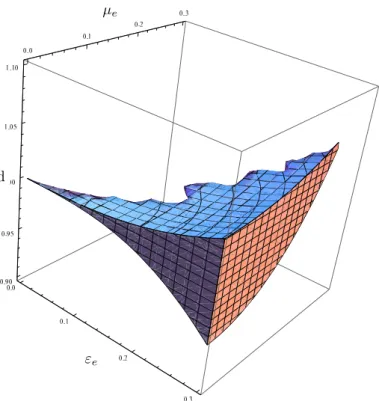
The asymmetric vibration offers the stabilization an essentially greater chance than the symmetric one: the acceleration can be a prescribed fixed value. Math- ematically formulating, for every µ¯e (0≤ µ¯e< √
2/2) there exist d¯≥1 and
d
εe
µe
Figure 3: A part of stability region.
¯
ε(k)e (¯ε(k)e → ∞as k→ ∞)such that equations (9) with parameters ε¯(k)e ,µ¯e,d¯ are strongly stable.
4 Periodic motions of the inverted pendulum
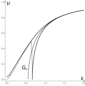
In the previous chapter we gave an estimation for the global stability map. Now, our aim to give the exact stability zones on the parameter plane introduced by Arnold [1], constructing2T- and4T-periodic solutions of the equation of motion with2T-periodic coefficient. As we know, the curves which correspond to these periodic solutions define the boundary of stability zone.
In the present chapter we study the pendulum whose suspension point vi- brates vertically under the influence of a symmetric effect. To this end, we consider the step function (8) as the acceleration of the excitation of suspension point of the pendulum. For the sake of simplicity, during this chapter, this acceleration function is2T-periodic. As in the case of problem of swinging, we transform the equation (9) to a discrete impulsive system, so we can use the phase trajectory to construct the periodic solutions of (9).
Our considerations show that2T- or4T-periodic trajectories can start only from points which are near the stable subspace y =−x. Restricting ourselves
these trajectories we can give necessary and sufficient conditions for the existence of the periodic solutions.
Theorem 4.1. There is a solution of (9) of period2T if and only if there are positive constantsA andT in (8)and a non-negative integer k such that either
2 arctan
DeωhT −1 eωhT + 1
+ 2kπ=ωeT, (16)
or
2 arctan
DeωhT+ 1 eωhT−1
+ (2k+ 1)π=ωeT. (17) Theorem 4.2. There is such a 4T-periodic solution of (9) which is not 2T- periodic if and only if there are positive constants A and T in (8) and a non- negative integer k such that either
2 arctan
DeωhT−1 eωhT+ 1
+ (2k+ 1)π=ωeT, (18) or
2 arctan
DeωhT + 1 eωhT −1
+ 2kπ=ωeT. (19)
So, now, we can describe the exact stability map and we can compare this with the estimated result. Figure 4 shows this situation. The first stability zone is located along the curveG0, in other words, this curve is the backbone of the first Arnold’s tongue.
Figure 4: The estimated and the exact stability zone
References
[1] V. I. Arnold, Ordinary Differential Equations, Springer-Verlag, Berlin, 2006.
[2] D. J. Acheson, T. Mullin, Upside-down pendulums, Nature, 366(2004), 215–216.
[3] J. Barrow, 100 alapvető dolog a matematikáról és a művészetről, amiről nem tudtuk, hogy nem tudjuk, Akkord Kiadó Kft, 2015.
[4] J. A. Blackburn, H. J. T. Smith and N. Gronbeck-Jensen, Stability and Hopf bifurcation in an inverted pendulum, Amer. J. Physics, 60(1992), 903–908.
[5] H. Broer, M. Levi, Geometrical aspects of stability theory for Hill’s equa- tions,Arch. Rational Mech. Anal.,131(1995), 225–240.
[6] H. Broer, C. Simo, Resonance Tongues in Hill’s Equations; A Geometric Approach, J. Differential Equations,166(2000), 290–327.
[7] E. Butikov, An improved criterion for Kapitza’s pendulum, J. Phys. A:
Math. Theor.,44(2011), 1–16.
[8] C. Chicone,Ordinary Differential Equations with Applications, Springer- Verlag, New York, 1999.
[9] L. Csizmadia, L. Hatvani, An extension of the Levi-Weckesser method to the stabilization of the inverted pendulum under gravity, Meccanica, 49(2014), 1091–1100.
[10] L. Csizmadia, L. Hatvani, On a linear model of swinging with a periodic step function coefficient,Acta Sci. Math. (Szeged),81(2015), 483–502.
[11] L. Csizmadia, L. Hatvani, On the existence of periodic motions of the excited inverted pendulum by elementary methods (submitted).
[12] S. Csörgő, L. Hatvani, Stability properties of solutions of linear second or- der differential equations with random coefficients, J. Differential Equa- tions,248(2010), no. 1, 21–49.
[13] A. M. Formal’skii, On the stabilization of an inverted pendulum with a fixed or moving suspension point, Dokl. Akad. Nauk, 406(2006), no. 2, 175–179.
[14] J. Hale, Ordinary Differential Equations, Wiley-Interscience, New York, 1969.
[15] P. Hartman, Ordinary Differential Equations, Birkhäuser, Boston, 2nd edn., 1982.
[16] L. Hatvani, On the existence of a small solution to linear second order differential equations with step function coefficients,Dynam. Contin. Dis- crete Impuls. Systems, 4(1998), 321–330.
[17] L. Hatvani, An elementary method for the study of Meissner’s equation and its application to proving the Oscillation Theorem, Acta Sci. Math., 79(2013), no. 1–2, 87–105.
[18] L. Hatvani, On the parametrically excited pendulum equation with a square wave coefficient, Internat. J. Non-Linear Mech., 77(2015), 172–
182.
[19] L. Hatvani, On small solutions of second order linear differential equa- tions with non-monotonous random coefficients,Acta Sci. Math. (Szeged), 68(2002), 705–725.
[20] L. Hatvani, L. Stachó, On small solutions of second order differential equa- tions with random coefficients, Arch. Math. (Brno), Equadiff 9 (Brno, 1997),34(1998), 119–126.
[21] G. W. Hill, On the part of the motion of the lunar perigee which is a function of the mean motions of the sun and moon, Acta Mathematica, 12(1886), Vol. 8, 1–36.
[22] H. Hochstadt, A special Hill’s equation with discontinuous coefficients, Amer. Math. Monthly, 70(1963), 18–26.
[23] P. L. Kapitsa, Dynamical stability of a pendulum when its point of sus- pension viberates, Zh. Eksper. Teoret. Fiz.,21(1951) (Russian)
[24] P. L. Kapitsa, Pendulum with a vibrating suspension, Uspekhi Fiz. Nauk, 44(1951) (Russian)
[25] L. D. Landau, E. M. Lifshitz, Mechanics, Course of Theoretical Physics, Vol. 1, Elsevier, Amsterdam, 1976.
[26] M. Levi, Stability of the inverted pendulum - a topological explanation, SIAM Rev.,30(1988), 639–644.
[27] M. Levi, Geometry of Kapitsa’ potentials,Nonlinearity,11(1998), 1365–
1368.
[28] M. Levi, W. Weckesser, Stabilization of the inverted, linearized pendulum by high frequency vibrations,SIAM Rev.,37(1995), 219–223.
[29] W. Magnus, S. Winkler, Hill’s equation, Dover Publications, Inc., New York, 1979.
[30] J. Meixner, F.W. Schäfke, Mathieusche Funktionen und Sphäroidfunktio- nen, Springer, 1954.
[31] E. Meissner, Über Schüttel-schwingungen in Systemen mit Periodisch Veränderlicher Elastizität, Schweizer Bauzeitung,72(1918), no. 10, 95–
98.
[32] D. R. Merkin, Introduction to the Theory of Stability, Springer-Verlag, 1997.
[33] A. A. Seyranian and A. P. Seyranian, The stability of an inverted pendu- lum with a vibrating suspension point, J. Appl. Math. Mech., 70(2006), 754–761.
[34] A. Stephenson, On an induced stability,Phil. Mag., Vol. 15.6(1908), 233–
236.
[35] A. Stephenson, On a new type of dynamical stability,Manchester Mem- oirs,52(1908), 1–10.
[36] G. Stépán, Mikrokáosz,Természet Világa,135(2004), 60–64.
[37] B. Van der Pol, M.J. O. Strutt, On the stability of the solutions of Math- ieu’s equation,The London, Edinburgh and Dublin Phil. Mag., 7th Series 5(1928), 18–38.