Adaptive Step Size Control for Hybrid CT Simulation without Rollback

(1)

Adaptive Step Size Control

for Hybrid CT Simulation without Rollback

Rebeka Farkas^1,2,3 Gábor Bergmann^1,2,3 Ákos Horváth^1,3

1Department of Measurement and Information Systems, Budapest University of Technology and Economics, Hungary,{farkasr,ahorvath,bergmann}@mit.bme.hu

2MTA-BME Lendület Cyber-Physical Systems Research Group

3IncQuery Labs Ltd, Hungary

Abstract

The Hybrid CT approach for simulating cyber-physical systems uses continuous time simulation and provides wrappers for discrete event components that implement the required interfaces. Besides the general obstacles of continuous time simulation, Hybrid CT introduces new challenges, such as creating wrappers, detecting discrete events (with minimal latency), and finding the correct bal- ance between the simulation step sizes required by different components.

We propose an adaptive step size controller that uses high level information of the model and the simulation (e.g. types of components, critical values of variables) to adjust the step size based on the possibility of the detection of a discrete event in the following step. Besides overcom- ing the challenges of Hybrid CT simulation the component also improves threshold-crossing detection. The proposed approach does not require step rejection (rollback), that discrete event components often fail to support.

In this paper we present the step size controller, demonstrate its usability on industrial case studies and evaluate the component both theoretically and based on measure- ments performed on our implementation that was integrated to the OMSimulator. We show that adaptive step size control can be used to bridge the gap between continuous time and discrete event simulation.

Keywords: hybrid CT simulation, step size control

1 Introduction

Hybrid systems demonstrate both discrete and continuous behaviour which makes their simulation challenging. A possible approach isHybrid CTthat usescontinuous time simulation and provides wrappers for discrete event components (as opposed toHybrid DEsimulation where continuous time components are adjusted so discrete event simulation can be used).

The OMSimulator developed by the Open Source Mod- elica Consortium (OSMC) uses Hybrid CT simulation based on the Functional Mock-up Interface (FMI) standard (Blochwitz et al., 2012) that defines a centralized architecture for simulation, where each component of the system (the so-called Functional Mock-up Units, FMUs)

is simulated on its own with amaster simulator controlling the process.

Despite the fact that there are proper approaches to create FMUs from discrete event components, the co- simulation of continuous-time and discrete-event blocks is still in its early phases. From a simulation point of view, one of the main differences between the two types of components is the simulation step size: continuous systems are simulated by periodically calculating the value of the variables with relatively large step sizes (measured in seconds) but discrete event-based systems operate irregularly and their simulation requires smaller steps (measured in nanoseconds) since discrete events can trigger other discrete events (almost) instantly. It is possible to simulate continuous-time models with smaller step sizes (in fact, it yields more accurate results), but it is inefficient (often preventing industrial application) and mostly unnecessary as events occur rarely. The sporadic occurrence of discrete events raises the need foradaptive step size control.

We propose an adaptive step size control approach to overcome the difficulties of hybrid CT simulation. The proposed solution requires the user to select the variables that are used to model event-based behaviour and adjusts the step size when their values change. Moreover, our approach can also be used to increase the accuracy of threshold-crossing detectionand location (which is an important aspect of hybrid simulation) without the need for rejecting steps (rollbacks).

This paper is organized as follows: section 2 presents some background knowledge on the challenges of Hy- brid CT simulation, section 3 lists the related work, section 4 presents the proposed step size controller, section 5 demonstrates its applicability, section 6 evaluates its use- fulness and section 7 concludes the paper.

2 Preliminaries

2.1 Running example: Thermostat

In this paper we use an advanced version of the commonly usedthermostat example to illustrate the presented con- cepts. The thermostat example describes a room with a thermostat keeping the temperature near some target temperature (with a given tolerance) that is given by a user

(2)

and can change through time. In addition we introduce a monitoring system to ensure that the thermostat operates correctly.

The monitoring system consists of three local monitors and each of them is responsible for a component of the heating system: the heating component, the heat sen- sor, and the thermostat. The monitoring system is con- trolled by a central monitor that communicates with the local monitors via messages to check wether the system is working correctly. Such a check is performed periodically every three minutes and each time before turning the heating on.

In the simulated scenario, the temperature initiates from 20^◦C with the target temperature set to 22^◦C. Originally the hysteresis is 3^◦C, but set to 2.5^◦C after half an hour.

The temperature of the environment is 0^◦C – that is, when the heating system is not activated the temperature of the room is decreasing towards 0^◦C. Initially, the thermostat is turned off but it is turned on after 10 seconds.

2.2 FMI-based hybrid co-simulation

The FMI standard for co-simulation makes it possible to simulate a system containing various components described by different types of models that require different ways of simulation. Co-simulation requires that each model is encapsulated with an appropriate simulator making an FMU which implements an interface through which the master simulatorcan control the simulation. In addition, the FMU also contains an XML-based model description file, with high level information about the model and additional information, such as theDefaultExperiment element that contains the default values of basic simulation parameters (e.g. stop time, relative tolerance, step size).

The modular architecture of FMI-based simulation makes it appropriate for hybrid co-simulation where the two types of components are the discrete event and the countinuous time components. Additionally, neither the model nor the simulator internal data need to be accessed, which makes FMI-based co-simulation industrially applicable.

OMSimulator is an FMI-based simulator for cyber- physical systems, developed by the OMSC. In order to simulate, the architecture must be defined (input and output ports must be coupled) and configuration data must be provided, e.g. simulation step size, tolerance, duration (the values given by theDefaultExperimentmay differ in each FMUs). After initialization the simulation is performed by alternating two types of steps: in asimulation stepthe master simulator instructs all FMUs to perform a step of the given step size, and in acommunication stepthe output values of the source components of the connections are passed as the input values of the corresponding target components. Simulation terminates after a given duration.

ExampleIn case of the thermostat example, we created the following FMUs.

• The Thermostat FMU contains a discrete event-

Room FMU

Thermostat FMU

Local monitor FMU 1

Local monitor FMU 2

Local monitor FMU 3

Central monitor

FMU Messages Settings, temperature,

heating control

Monitoring information Figure 1.Thermostat FMU architecture

based model describing the operation of the thermostat. The inputs of the thermostat include the settings and the current temperature.

• The Room FMU contains a continuous model describing the characteristics of the physical world, including the temperature and the user that provides the settings of the thermostat. The user operations are pre-defined and the temperature is calculated based on the heating.

• The (discrete event-based) models of the each monitors are provided in separate FMUs. The monitors get the same inputs as the thermostat and check if the operations of the thermostat are correct.

Accordingly theThermostatand theRoomFMUs are connected, and the monitors are connected to both both of them are connected to each monitors. The complete architecture can be seen in Figure 1.

2.3 Simulation challenges

One of the most important requirement of simulation is accuracy: while it is theoretically impossible to calculate accurate values, there are many ways to calculate an over- approximation of the error and to keep it below a given amount (Viel, 2014; Arnold et al., 2014a,b). The other important requirement is efficiency and – as usual – the two requirements contradict.

In case of iterative methods accuracy can be improved by increasing the number of iterations during a simulation step. In practice the iterations required to comply with the desired tolerance can result in an impermissibly large runtime which makes non-iterative methods favoured in case of co-simulation.

In case of non-iterative methods efficiency depends on the number of steps performed (hence, larger step size yields more efficient simulation) and accuracy depends on the size of the steps (smaller step size yields more accurate results). As an optimization, master algorithms often use rollbacks (the rejection of one or more steps) when the simulation error is above the tolerance and then re- simulate with smaller step sizes. Rollbacks have other ad-

(3)

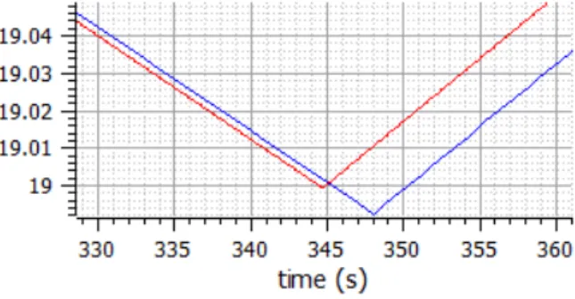
Figure 2.Simulation error caused by step size

vantages, e.g. in case of the so-calledthreshold-crossing detectionproblem, where it has to be detected (and lo- cated) when a given variable reaches a certain value.

Introducing discrete event components into a continuous time environment raises a new challenge, as it becomes more important to detect events with minimal latency. While this problem can also be solved with rollbacks (Galtier et al., 2015) many discrete event FMUs can not handle rollbacks and therefore the only way to ensure the events are detected in time is to use smaller step sizes that makes simulation intractably expensive. It is also possible to attempt topredictevents (Guermazi et al., 2016).

Example: In case of the thermostat example thedetec- tion of discrete eventsbecomes important with the monitoring system: when the central monitor gathers information to check if the thermostat works correctly, messages are passed between the monitors. This process is fast and in order to simulate it accurately, the simulation step sizes have to be small, as a number of discrete events (the messages) are triggered by each other, therefore at most one of these events occur in each simulation step. This communication between the monitors takes place when the heating has to be turned on as well as every three minutes when the periodical checks are performed. The former scenario introduces athreshold-crossing detectionchallenge: it is important to detect when the temperature exceeds the bounds of the target interval (initially 19^◦C and 25^◦C), and the periodical checks raise the need forevent prediction.

In order to demonstrate the importance of keeping the latency minimal, we have simulated the first time the temperature falls below 19^◦C in the thermostat example (ex- cluding the monitor components) with constant step sizes of 0.1 s and 0.01 s. The threshold-crossing happens about 344 seconds from initialization. The results are shown in Figure 2, where thexaxis represents the (simulated) time and theyaxis represents the simulated temperature. The red line denotes the results of simulation with the smaller step size and blue line corresponds to the larger step size.

Before the threshold-crossing the two simulation produces similar results – with an exception of an initialization off- set (explained in subsection 6.2). However, after the temperature decreases below 19^◦C the two simulations pro- duce significantly different results. The reason behind this

is that because of the larger step sizes both the threshold- crossing and the discrete reactions are detected with latency. Because of this, in case of the smaller step size the temperature raises over 19^◦C in less than a second, while in case of the other simulation it takes almost five seconds which is a simulation error caused purely by event detection latency introduced by the large step sizes.

3 Related work

Discrete components in simulation There is extensive existing research on introducing discrete event components to continuous time environments. In (Guermazi et al., 2016) the discrete event components are integrated in the continuous time simulation workflow as a white box, and the communication intervals are adjusted to detect events based on internal information. In (Galtier et al., 2015) rollbacks are used: when an event is detected, the last step is rejected and the simulation step size is adjusted to the minimum amount to locate it. In (Franke et al., 2017) discrete time simulation is supported by introduc- ingclocksand correspondingclocked variablesthat only have values when the clock ticks.

Step size control There are many adaptive step size control approaches for enhancing the performance of the simulation (Schierz et al., 2012; Viel, 2014), but most of them rely on internal data and step rejection, with the exception of (Busch and Schweizer, 2011) that uses a non- iterative predictor/corrector error estimator. Adaptive step size control can also be used for threshold-crossing detection and location (Esposito et al., 2001) .

Since the presented algorithms all focus on finding the largest possible step size, it is theoretically possible to combine them.

4 Adaptive step size control for Hybrid CT simulation

4.1 Overview of the approach The approach is illustrated in Figure 3.

General idea The step size controller unit is a component of the master simulator, invoked immediately before performing a simulation step, as depicted in Figure 3a.

The size of the next simulation step is calculated based on a number of influencing factors, such as values of variables getting near to thresholds, expected occurrence of events, expected event-responses, etc. These parameters are pre-defined in a data structure that we call the sensitivity model, that can be considered a configuration parameter of the simulation. Afterwards, the simulation step is performed with the calculated step size. The simulation step is followed by a communication step which is followed by the step size calculation preparing the next simulation step and so on.

Architecture The step size controller can be a component of the master simulator or an additional layer con-

(4)

Master simulator

FMU FMU FMU ...

Adaptive step size controller

Initialization

Master simulator Communication step

Simulation step Step size calculation (a)Master simulation algorithm

Master simulator

FMU FMU FMU ...

Adaptive step size controller Configuration

Sensitivity model Global

parameters (e.g. stopTime)

(b)Architecture Figure 3.Overview of approach

trolling it. The required sensitivity model is an input of the component (or the simulator) – in the current implementation the complete sensitivity model has to be provided together, altough it would be more practical to provide the FMU-specific elements individually, encapsulated with the corresponding FMUs (see subsection 6.2).

The architecture can be seen in Figure 3b.

Information to provide In case of FMI-based co- simulation of a large-scale system integration project, the FMUs can originate from different stakeholders who may wish to safeguard their intellectual property. While the sensitivity model does require some information on the operation, this information could also be derived by con- ducting a limited number of preliminary simulation runs with large (fix) step sizes (see subsection 5.2). Therefore the sensitivity model is a convenient compromise between making the models public in order to simulate them accurately and hiding the models and simulate with impracti- cably small step sizes.

4.2 Sensitivity model

The sensitivity model parametrizes the adaptive step size control approach. It describes the critical scenarios that require accurate calculations or detecting discrete events with low latency – that is, the scenarios where it is important to set the step size small.

In case of FMI-based co-simulation the numerical accuracy is ensured by the internal simulators of the FMUs,

but in order to detect a discrete event precisely, the event has to occur at the last moment of the simulation step, otherwise the event is detected with latency.

4.2.1 Described scenarios

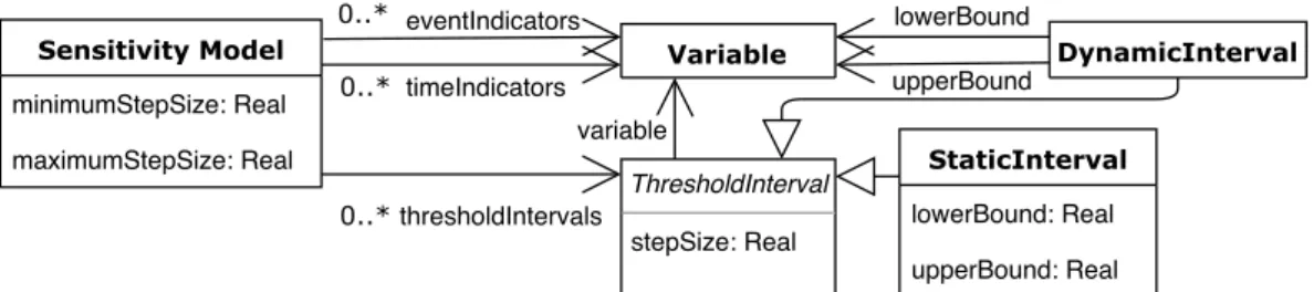
The sensitivity model was created to describe various scenarios where the step size need to be adjusted. The data structure of the proposed sensitivity model can be seen in Figure 4. The described scenarios can be classified as follows.

Event reactions Discrete events may trigger other discrete events that have to be simulated with minimal latency. In order to identify these scenarios, a set ofevent indicators– i.e. variables where the change of the value represent an event – have to be declared. During simulation when an event is detected, the step size is set to minimal, so that the reactions can be simulated accurately.

Example: In order to avoid the latencies during the se- quences of discrete events during the simulation of the thermostat, all variables representing messages should be included in the set of event indicators. However, this solution does not prevent the latency in the detection of the first message.

Timed events Discrete events may be triggered by the elapse of time. In order to perform a simulation step so that the discrete event is simulated without significant latency, they have to be predicted - i.e. the sensitivity model has to store when to expect an event. A set of variables, calledtime indicatorscan be given that each indicate when an event will be fired. The values of the variables can be changed during simulation so periodical events only require one indicator variable.

Example: It can be predicted when the central monitor initiates the periodical check based on the variable the component uses for timing the first message.

Threshold-crossing Discrete events may be triggered by continuous variables crossing a given threshold. In order to facilitate the detection of such scenarios with minimal latency the sensitivity model allows the description of auxiliarythreshold intervalsfor the variable with corresponding step sizes. Intuitively, the auxiliary intervals should describe when the value isclose to the threshold and a corresponding step size should be small enough to detect it. Accordingly, the step size controller does not guarantee to precisely detect when a value of a signal gets inside an interval (hence the interval should be appropri- ately large) but as soon as it is detected, the step size is adjusted accordingly. This way if the limits of the auxiliary interval are appropriate considering the behaviour of the system, the threshold-crossing can be detected with low latency.

Example: In case of the threshold-crossing depicted in Figure 2 the temperature decreases less than 0.003^◦C in a second, therefore any upper bound over 19.003^◦C and lower bound below 19^◦C guarantees that a simulation with a step size of 1 second will surely include a com-

(5)

Sensitivity Model minimumStepSize: Real maximumStepSize: Real

0..* eventIndicators

StaticInterval lowerBound: Real upperBound: Real ThresholdInterval

stepSize: Real Variable 0..* timeIndicators

variable

0..*thresholdIntervals

lowerBound upperBound

DynamicInterval

Figure 4.Sensitivity model data structure

munication step where the temperature is in the interval but more than 19^◦C. If the step size corresponding to the threshold interval is 0.1 second, then by the time the target threshold-crossing happens the step size will be set to 0.1 second and the threshold-crossing will be detected with a smaller latency. (Naturally, choosing the appropriate upper boundbeforesimulation is more difficult and requires domain knowledge.)

4.2.2 Dynamic parameters

Parameters of the model (execution of timed events, thresholds) can be declared both statically and by assign- ing a variable of the FMU whose value determines the current value of the parameter – the latter can be useful e.g.

for declaring the next occurrence of a timed event or when the important threshold to cross can change through time.

Example: The constant threshold-interval in the previous example only facilitates the threshold-crossing detection until the hysteresis changes. In order to create a general solution, additional variables have to be introduced to the model, e.g. instead of the constant upper bound 19.003^◦C an additional variablevaddcan be used with the valuevadd=vtrg−vhys+0.01^◦C wherevtrg is the target temperaturevhysis the hysteresis and the constant was increased to ensure the interval is large enough.

As demonstrated by the example, additional variables often have to be created in order to describe dynamic parameters. While it is not always possible to modify the FMUs since they are generated, but it is always possible to create an additional FMU with the additional variables that takes the outputs of other FMUs as inputs.

It is important to mention that the sensitivity model de- scribesexpectedscenarios – it does not make a difference during simulation whether the expected events are actually detected, which makes it applicable for non-deterministic models. However, the unnecessary adjustments cause the simulation to be less efficient than it could be if the sensitivity model was more precise.

4.2.3 Minimal and maximal values

As a reference, the minimum and the maximum value of the step size has to be declared before the simulation. It is guaranteed that during simulation the step size will always be between the minimum and the maximum value (except for the very last step that may be smaller than the

t

t-0.05 t+0.05 t-0.05 t t+0.05

Minimal step size

Latency Event

indicator Output

(a)Event t

t-0.05 t+0.05 t-0.05 t t+0.05

Minimal step size

Latency Event

indicator Output

(b)Event detection Figure 5.Event detection latency example

lower bound). Generally, the main reason for the lower bound is to avoid Zeno behaviour that could otherwise be easy to cause (e.g. it is possible to schedule a sequence of timed events, always with half as much delay as the last one). However, in case of Hybrid CT simulation the lower bound is the guaranteed maximal delay of detecting a timed event, as well as the guaranteed delay between a sequence of discrete events triggered by each other. The upper bound becomes significant when there is no discrete event to expect in the next step – in this case, the step size is set to the given maximum value.

Example In order to demonstrate the significance of the minimal step size, consider the periodical check performed by the central monitor. Let us suppose the next check is scheduled at time stampt however, because of an active threshold-interval, the current step size is 0.15 s, the simulation time after the last step ist−0.05 s and the minimal possible step size is 0.1 s. Since the size of the next simulation step has to be at least 0.1 s the the event will be detected att+0.05 s. The latency is illustrated in Figure 5.

The event initiates a sequence of discrete events (responses) and if the event indicators are defined appropri- ately in the sensitivity model then the step size stays at the minimal value during the simulation of the event sequence.

4.2.4 IP protection concerns

In an industrial environment it is possible that the model constitutes confidential intellectual property and using the

(6)

step size controller would require disclosing some of the restricted information in the sensitivity model.

In this case the step size controller has to be used differ- ently: in order to protect intellectual property, the model needs to be modified so that the critical scenarios are iden- tified within the FMU. This can be achieved using an auxiliary variable representing the critical scenarios and creating corresponding threshold intervals in the sensitivity model.

Example:Suppose there is a critical scenario that must be simulated precisely. Instead of providing a detailed sensitivity model, an auxiliary variablev can be used to identify the scenario – e.g. v=1 during the scenario andv=0 otherwise. The corresponding interval can be 0.5≤v≤1.5 and the corresponding step size can be the minimal value. This way, when the critical scenario is detected (within the FMU)vis set to 1 and the step size controller adjusts the step size to the minimal value.

4.3 Algorithm

In order to calculate the size of the simulation steps, the latest values of event indicators have to be stored. After a communication step, the size of the next simulation step is calculated based on the detected events, the scheduled timed events and the threshold-crossing intervals. Each element of the sensitivity model defines an upper bound on the size of the next step (including the global maximum step size), therefore the actual value of the next step should be the minimum of the given upper bounds (unless it is smaller than the possible minimal value).

An event can be detected by checking if the current value of the corresponding event indicator differs from its previous value. When an event is detected the step size has to be set to the minimal possible value. The stored (previous) values of event indicators always have to be updated, but when an event is detected, no additional calculations are necessary as the step size will certainly be set to the minimal possible amount.

In case when no event is detected the time indicators and the threshold intervals have to be checked. If a value of a time indicator is less than the current simulation time t, it is irrelevant. The time indicator with the smallest valuet_min>t denotes the next possible timed event. In order to detect the event precisely the next step can not exceed the differencetmin−t, except if it is less than the defined minimum.

The upper bound on the next step based on the threshold intervals can be derived by checking the corresponding variables – if the value of a variable is within the bounds of one of its corresponding auxiliary intervals, the next step can not exceed the corresponding step size described in the sensitivity model.

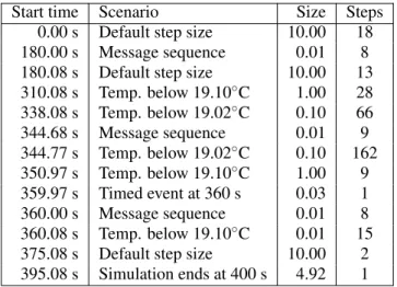
Example: Let us demonstrate the simulation using adaptive step size control on the thermostat model with the sensitivity model describing the scenarios discussed before and the minimal step size set to 0.01 s and the maximal step size set to 10 seconds. (The bounds of the step

Table 1.Adaptive step sizes of the Thermostat

Start time Scenario Size Steps

0.00 s Default step size 10.00 18 180.00 s Message sequence 0.01 8 180.08 s Default step size 10.00 13 310.08 s Temp. below 19.10^◦C 1.00 28 338.08 s Temp. below 19.02^◦C 0.10 66 344.68 s Message sequence 0.01 9 344.77 s Temp. below 19.02^◦C 0.10 162 350.97 s Temp. below 19.10^◦C 1.00 9 359.97 s Timed event at 360 s 0.03 1 360.00 s Message sequence 0.01 8 360.08 s Temp. below 19.10^◦C 0.01 15 375.08 s Default step size 10.00 2 395.08 s Simulation ends at 400 s 4.92 1

size are intentionally unrealistic to demonstrate the operation of the step size control.) The intervals for the threshold crossings are set so that when the difference between the current threshold is less than 0.1^◦C, the step size is set to 1.0 s and when it is less than 0.02^◦C, the step size is set to 0.1 second. The model is simulated for 400 seconds.

The step sizes are shown in Table 1.

The simulation begins with the maximal step size. The first periodical check happens to be scheduled exactly at the end of the 18th step, therefore, the step size does not have to be adjusted. However, as soon as the first message is detected, the sequence of discrete events caused by the messages is simulated with minimal latency.

In case of the checks caused by the temperature decreasing below 19^◦C, the first discrete event – the state transition of the thermostat – is detected with (relatively) high latency: the current step size to the corresponding interval, namely 0.1 s. After that, the monitors send the same eight messages which is why there is one more event in this sequence, than in the ones representing the messages passed during the timed checks.

In conclusion the simulation takes 340 steps, which is 99% less than what it takes to simulate it with constant step size of 0.1 s (which would take 40 000 steps) but the results are more precise.

5 Experimental evaluation

We have integrated the proposed adaptive step size controller component in the OMSimulator¹and run measure- ments on case studies with constant steps of different step sizes as well as using adaptive step size control. In order to find out how the step size controller affects performance we measured the runtime and then analysed the differences between the efficiency and the results of corresponding simulations.

(7)

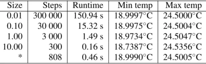
Table 2.Simulation performance of the Thermostat example

Size Steps Runtime Min temp Max temp 0.01 300 000 150.94 s 18.9997^◦C 24.5000^◦C 0.10 30 000 15.32 s 18.9975^◦C 24.5004^◦C 1.00 3 000 1.49 s 18.9734^◦C 24.5047^◦C 10.00 300 0.16 s 18.7387^◦C 24.5356^◦C

* 808 0.46 s 18.9990^◦C 24.5005^◦C

5.1 Thermostat

The sensitivity model for the Thermostat was presented in section 4. We performed the simulation with various constant step sizes as well as with the step size controller.

Each time 3000 seconds were simulated. The results are shown in Table 2. The columns of the table contain the step size, the number of steps performed, the runtime of the simulation, and the minimal and the maximal simulated temperature (respectively). The * in the first cell of the last row represents that the simulation includes various step sizes, as chosen by our adaptive algorithm. The simulation with adaptive step size control resulted in 144 steps of 0.01 s, 282 steps of 0.1 s, 93 steps of 1 s, 275 steps of 10 s and 13 steps of other sizes.

In the simulated scenario, the target temperature is 22^◦C with initially 3^◦C tolerance (which is why the minimal value is just below 19^◦C) that is later set to 2.5^◦C by the user (which is why the maximal value is just above 24.5^◦C). The results show, that – in case of constant step sizes – an order of magnitude difference in the step sizes yields an order of magnitude difference between the expected and the simulated extreme values. However, in case of adaptive step size control, the difference is almost as small as in case of the 0.01 s steps while the simulation was almost as fast as in case of the 10 s steps.

5.2 Sherpa Automotive demonstrator

The Sherpa Automotive demonstrator is one of the industrial models in the OpenCPS project²that served as a basis for required improvements of the simulator.

The case study contains the models representing the mobility aspects of the system presented in (Mokukcu et al., 2017). The physical aspects of a hybrid electric vehicle are simulated to determine the amount of energy required for the vehicle to move with the required speed.

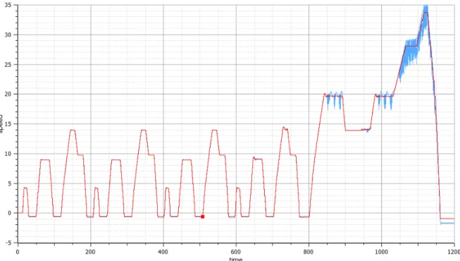
The simulated scenario is 1200 time units and the default step size is 0.01. We have performed the simulation with constant step sizes of 0.1 and 0.01. The simulated speed of the vehicle is depicted in Figure 6. Up to 800 time units the results are similar: the largest difference between the result of the simulation with the small (red) and the large (blue) step size is less than 0.55. The biggest differences

1https://github.com/OpenModelica/OMSimulator

2ITEA3, OpenCPS: Open Cyber-Physical System Model-Driven Certified Development http://www.opencps.eu

appear near to the local minimum and local maximum values. In the remaining part of the simulation the differences are much larger (14.0) and additional high frequency sine components appear. The unstable oscillating waveforms show that a step size of 0.1 is too large for accurate simulation.

The goal of adaptive step size control is to improve simulation performance by using larger step sizes where it does not affect precision. After studying the results we have created a simple sensitivity model: braking is considered a discrete event, therefore the the signal representing the brake position is used as an event indicator, and in order to avoid the additional sine components, threshold intervals are used on the variable representing the target speed.

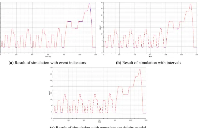
We run the simulation, with 0.1 as maximal and 0.01 as minimal step size three times with the event indicator and the intervals individually and combined. The results can be seen in Figure 7. The runtimes and an evaluation of all performed simulations are shown in Table 3. The Diff column of the table denotes the maximum difference between the simulated speed of the vehicle and the speed simulated by the default simulation andDiff2denotes the maximal difference in the first 800 s of simulation time.

Using the brake as event indicators causes a runtime almost 90% smaller than that of the original simulation with step size 0.01 while reducing the error of the large step size simulation: in the first part the difference remained under 0.55 and the unstable oscillations of the results disappear decreasing the biggest difference to 2.8. However, some additional low frequency sine waveforms can still be seen.

Using the intervals (without event indicators) causes a runtime 40% smaller than the simulation with the small step sizes and reduces the error of the simulation with the large step sizes: in the first part the difference is less than 0.55 and the obscure parts of the result disappear decreasing the maximum of the difference to 0.7. However, one additional sine waveform remains.

Using both elements of the sensitivity model combines the advantages in accuracy as the results of the simulation are almost the same as that of the simulation with the small step size. However, the resulting runtime is larger than that of the simpler sensitivity models (though not as large as the runtime with a fixed small step size), since in each step the step size is the minimum of those in the previous cases.

The results show, that using the brake as event indicator increased the performance drastically while only introducing small simulation errors. The case study also demonstrated that intervals can be used to identify the critical scenarios.

(8)

Figure 6.Simulation results of automotive case study

Table 3.Simulation performance of the automotive case study

Events Intervals Small steps Large steps Total steps Runtime Diff Diff2 Remark

120 000 0 120 000 31.27 s – – Default simulation

0 12 000 12 000 3.59 s 14.0 0.55 Unstable oscillations

+ 688 11 932 12 620 3.90 s 2.8 0.54 Sine waveforms

+ 34 900 8 511 43 411 18.54 s 0.9 0.55 Sine waveform

+ + 35 005 8 500 43 505 18.81 s 0.7 0.54 Almost identical

6 Discussion

6.1 Limitations and opportunities

As demonstrated in section 5 adaptive step size control can be used to improve simulation performance. Step size control has been shown to be effective for event detection as well as decreasing runtime while preserving numerical accuracy.

Usability The sensitivity model for the adaptive step size controller requires domain knowledge (e.g. for event prediction), however, some parts of it (e.g. the step sizes assigned to the intervals for threshold-crossing detection) depend on the current simulation configuration. Since both domain-specific and simulation-specific knowledge are required, using the step size controller in its current form may cause difficulties in an industrial environment.

A possible solution can be separating the required information and creating the sensitivity model in a final step (see subsection 6.2).

Extensibility The proposed step size controller can be easily extended with additional functionalities: the core of the proposed approach is determining an upper bound of the size of the next step based on several approaches and then choosing the minimum of the calculated upper bounds – it is easy to introduce new analysis methods to the sensitivity model that determine upper bounds based on new aspects. For instance, the algorithm could be combined with the step size controller approach for numerical stability proposed in (Busch and Schweizer, 2011) or the threshold-crossing detection approach proposed in (Esposito et al., 2001).

Possible improvements The proposed solution only considers the possible events in the next step, which – as presented in subsection 4.2 – causes delays. The delays could be minimized using a lookahead method that includes more than one step in the calculation.

Example: In the previously referred example there is a communication step att−0.2 s. No event is expected in the next simulation step, therefore the next step size is set to 0.15 s. Att−0.05 s the event att is considered, but

(9)

(a)Result of simulation with event indicators (b)Result of simulation with intervals

(c)Result of simulation with complete sensitivity model

Figure 7.Results of simulating the automotive case study with step size control

since the minimal step size is 0.1 s the event is detected with latency. However, the delay can be prevented by tak- ing two consecutive steps of 0.1 s.

The threshold-crossing detection approach can also be improved by using an advanced solution that uses extrap- olation to analyse the possibility of threshold crossing and adjust the step size accordingly. This way it can be avoided to provide intervals and corresponding step sizes.

6.2 Lessons learnt

Implementation Throughout the OpenCPS project we have simulated FMUs from various sources, such as OMEdit, Dymola, Simulink, etc. and we have discovered that some FMUs do not comply with the FMI standard completely. As mentioned before, sometimes FMUs can not perform rollbacks. Additionally, in case of the thermostat example the changes in the step sizes introduced odd slopes that later turned out to be caused by the fact that certain defective FMU implementations always perform the step with the previous step size. The difference between the values of the decreasing phase of Figure 2 is caused by the same phenomenon: in the first simulation step (not depicted in the figure) the value does not change and the decrease of the temperature starts in the second simulation step, which is at 0.1 s in one case (denoted by the blue line) and 0.01 s in the other. The time shift causes the difference between the values. This shows that the FMUs must be prepared in order to use adaptive step size control effectively.

Error approximation Currently there are no approxi- mations for the error of the simulation, other than that of the internal simulators of the FMUs. However, – as demonstrated in Figure 5 – discrete events can introduce new types of errors besides numerical stability. The calculation of simulation errors resulting from hybrid co- simulation is a complex theoretical problem and we believe it is an area worth exploring.

Simulation configuration The sensitivity model requires data that can be difficult to acquire, especially when the FMUs to co-simulate originate from different stakeholders. While the DefaultExperiment element of the model description file contains simulation-specific information, it only specifies configuration data for simulation with constant step size. Moreover, from a hybrid co-simulation point of view, there are few ways to provide discrete system-specific information in the model description file. A notable exception is the variability at- tribute ofScalarVariableelements that can be set todis- crete thereby denoting an event indicator. However, in case of FMI for co-simulation, timed events and relevant threshold-crossings can not be specified.

Accordingly, in the current implementation the information stored in the sensitivity model is provided by the user as an input of the simulator. However, we believe it would be beneficial to make it possible to provide information specific to discrete/hybrid systems and configuration parameters for simulation with variable step size in the model description file.

(10)

7 Conclusions

In this paper we presented a step size controller approach that improves continuous time simulation of discrete event components. The core of the approach is the sensitivity model that describes the simulation scenarios where it is necessary to adjust the step size in order to simulate accurately. The sensitivity model can include se- quences of discrete events, timed events and intervals for threshold-crossing detection. The described scenarios can also change dynamically during simulation.

After each communication steps of the master algorithm, the size of the next simulation step is calculated based on the sensitivity model and the current values of variables. The presented method does not require rollbacks.

We have implemented the presented approach within OMSimulator and studied its applicability to the Thermo- stat example as well as an industrial case study. The results show that the step size controller provides a better compromise between simulation accuracy and efficiency than fixed step sizes by using small step sizes only when is required for simulation accuracy.

We have conducted experiments and found that the step size controller can bridge the gap between continuous time simulation and discrete event components, thereby im- proving simulation of cyber-physical systems.

Acknowledgement

This project was partially supported by the Hungarian National Research, Development and Innovation Office through the EUREKA_15-1-2016-0008 project as part of the international ITEA3 OpenCPS (14018) project. The authors would like to thank Magnus Eek, Lennart Ochel, Philippe Fiani and Krisztián Mócsai for their assistance in this research.

Gábor Bergmann was partially supported by the János Bolyai Research Scholarship of the Hungarian Academy of Sciences and by the ÚNKP-18-4 New National Excel- lence Program of the Ministry of Human Capacities.

References

Martin Arnold, Christoph Clauß, and Tom Schierz. Error analysis and error estimates for co-simulation in fmi for model exchange and co-simulation v2. 0. InProgress in Differential- Algebraic Equations, pages 107–125. Springer, 2014a.

Martin Arnold, Stefan Hante, and Markus A Köbis. Error analysis for co-simulation with force-displacement coupling.

PAMM, 14(1):43–44, 2014b.

Torsten Blochwitz, Martin Otter, Johan Akesson, Martin Arnold, Christoph Clauss, Hilding Elmqvist, Markus Friedrich, An- dreas Junghanns, Jakob Mauss, Dietmar Neumerkel, et al.

Functional mockup interface 2.0: The standard for tool in- dependent exchange of simulation models. InProceedings of the 9th International MODELICA Conference; September 3-5; 2012; Munich; Germany, number 076, pages 173–184.

Linköping University Electronic Press, 2012.

Martin Busch and Bernhard Schweizer. An explicit approach for controlling the macro-step size of co-simulation methods. Proceedings of The 7th European Nonlinear Dynamics, ENOC, pages 24–29, 2011.

Joel M Esposito, Vijay Kumar, and George J Pappas. Accurate event detection for simulating hybrid systems. In Interna- tional Workshop on Hybrid Systems: Computation and Con- trol, pages 204–217. Springer, 2001.

Rüdiger Franke, Sven Erik Mattsson, Martin Otter, Karl Wern- ersson, Hans Olsson, Lennart Ochel, and Torsten Blochwitz.

Discrete-time models for control applications with fmi. In Proceedings of the 12th International Modelica Conference, Prague, Czech Republic, May 15-17, 2017, number 132, pages 507–515. Linköping University Electronic Press, 2017.

Virginie Galtier, Stephane Vialle, Cherifa Dad, Jean-Philippe Tavella, Jean-Philippe Lam-Yee-Mui, and Gilles Plessis.

Fmi-based distributed multi-simulation with daccosim. In Proceedings of the Symposium on Theory of Modeling & Sim- ulation: DEVS Integrative M&S Symposium, pages 39–46.

Society for Computer Simulation International, 2015.

Sahar Guermazi, Saadia Dhouib, Arnaud Cuccuru, Camille Letavernier, and Sébastien Gérard. Integration of UML models in fmi-based co-simulation. InTMS/DEVS 2016, page 7.

ACM, 2016.

Mert Mokukcu, Philippe Fiani, Sylvain Chavanne, Lahsen Ait Taleb, Cristina VLAD, and Emmanuel Godoy. Control Architecture Modeling using Functional Energetic Method:

Demonstration on a Hybrid Electric Vehicle. In 14th In- ternational Conference on Informatics in Control, Automa- tion and Robotics (ICINCO), Madrid, Spain, July 2017.

doi:10.5220/0006413300450053. URL https://hal.

archives-ouvertes.fr/hal-01719924.

Tom Schierz, Martin Arnold, and Christoph Clauß. Co- simulation with communication step size control in an fmi compatible master algorithm. InProceedings of the 9th In- ternational MODELICA Conference; September 3-5; 2012;

Munich; Germany, number 076, pages 205–214. Linköping University Electronic Press, 2012.

Antoine Viel. Implementing stabilized co-simulation of strongly coupled systems using the functional mock-up interface 2.0.

InProceedings of the 10 th International Modelica Confer- ence; March 10-12; 2014; Lund; Sweden, number 096, pages 213–223. Linköping University Electronic Press, 2014.