An automated method for generating customizable cages using barycentric
coordinates
Ákos Tóth, Roland Kunkli
Faculty of Informatics, University of Debrecen, Debrecen, Hungary [toth.akos,kunkli.roland]@inf.unideb.hu
Submitted June 1, 2018 — Accepted November 9, 2018
Abstract
In computer graphics, we usually use cage-based deformation techniques to manipulate high-resolution 3D models in real time. The most time-con- suming task in cage-based deformation is the construction of the cage which surrounds the model to be deformed. In this paper, we introduce a novel method to generate cages for 3D triangulated models automatically. The desired number of the cage vertices and the distance between the cage and the input model are adjustable by the users. Our method generates a cage which envelops the model, then eliminates the intersections between them.
The result of the algorithm is a 3D triangulated mesh (called cage) which can be used for cage-based deformation techniques without any modifications.
Experimental results and demonstrative pictures show that our algorithm is effective for different types of 3D models.
Keywords:cage generation, cage-based deformation, mesh deformation MSC:68U05
1. Introduction
In modern computer graphics, one of the most important conditions to render a realistic animation scene is to use detailed, high-resolution 3D models. However, the direct manipulation of these models is very expensive and difficult; therefore, we can use different deformation techniques (e.g., Harmonic Coordinates [8], Mean doi: 10.33039/ami.2018.11.002
http://ami.uni-eszterhazy.hu
167
Value Coordinates [9], or Green Coordinates [12]) to reduce the computational cost of the real-time model manipulation.
These cage-based deformation methods [14] usually use a simplified, coarser triangle mesh—often called cage—to manipulate the model. The cage has to be closed and surround the model to be deformed, without any intersection. There- after, if we define a relationship between the cage and its interior with the help of barycentric coordinates, we can manipulate any complex object by moving the vertices of the cage in real time after a short pre-computation phase. In most cases, it is enough for us to use coarse cages with few vertices (e.g., collision detection), but thanks to the rapid evolution of the computing capacity, we can make finer modifications on the input model by using more detailed cages.
As of now, the cages are often constructed by the users manually which is a tiresome task and takes long time. Furthermore, when the topology of the original model is complex, the cage construction is hard by hand. Recently, there exist robust methods which can generate cages semi-automatically [10] or automatically [3, 15] for 3D models. These approaches use numeric methods for minimizing en- ergy functions which could lead to time-consuming computations. An automated method of Xian et al. [18] can construct coarse cages efficiently, but in some cases, it is not possible to generate sufficiently detailed cages. Thus, the required defor- mation is hardly feasible in these situations. Therefore, our goal was to provide an easily calculated, fast, and customizable method which can generate cages au- tomatically for 3D triangulated meshes.
In the next section, we give a short overview of cage-based deformation tech- niques and their properties. Then, in Section 3, we introduce previous works and recent results related to the topic. We highlight their main advantages and disad- vantages as well. In Section 4, we discuss our method in detail, while Section 5 presents the experimental results.
2. 3D model deformation techniques
Mesh deformation is a challenging process and an active research area in computer animation and geometric modeling. The effect of it must be very accurate and realistic, but at the same time, it must be easily changed to allow the designers to express their imaginative ideas.
The principal thing is that we need a flexible toolkit for mesh deformation to achieve the expected results easily. Many methods have been released in the last decades in this direction such as free-form deformation (FFD) [16], Radial Basis Functions (RBF) [2], generalized barycentric coordinates (GBC) [4], as-rigid-as- possible surface modeling [17], or skeleton and curve based deformation techniques [1, 19].
Character articulation—so-called rigging—also fulfills an essential role in the area of model deformation. It has some constraints that some of the methods men- tioned above cannot satisfy, like operating in real time. It may also be important to have a user-friendly and easy to use system for character deformations. Cage-based
deformation techniques can be used efficiently for this kind of purpose.
The first approaches in this area were born at the dawn of animated film pro- duction. The pioneers were Thomas W. Sederberg and Scott R. Parry. They defined the free-form deformation technique [16] which became popular because it offers intuitive control over the model with only a few lattice control points. The only constraint that the model has to fulfill is to be inside the control lattice. And besides, this method has some disadvantages: if the character is complex, the de- formation becomes challenging, and the lattice cannot fit to the model perfectly.
Consequently, new methods appeared which use cages that fit better to the char- acter shape, such as Mean Value Coordinates, Harmonic Coordinates, or Green Coordinates. In the next subsection, we recall the principles of them based on Nieto’s and Susín’s survey [14].
2.1. Fundamentals of cage-based deformations
Let us be given a cageC(any triangle mesh or a polyhedric mesh) which is closed and envelops the model to be deformed. Then we need to define a relationship between the cage and its inside volume, after that, the deformation of the cage will affect the interior object. This procedure allows us to manipulate any complex model inside the cage.
To define the previously mentioned relationship between the cage and its inte- rior, we can use barycentric coordinates which were first introduced by Möbius [13]
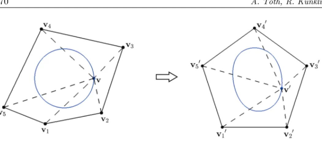
in 1827. If we place weightsw1,w2, andw3at the vertices of a triangle (v1,v2, and v3 respectively), then any pointvof the triangle can be obtained by the weighted sum of these vertices. The barycentric coordinates of pointv are the weightsw1, w2, andw3. The idea can be generalized, i.e., vcan be defined as the barycenter of the pointsv1, . . . ,vn if and only if
v=w1(v)v1+· · ·+wn(v)vn
w1(v) +· · ·+wn(v) . These barycentric coordinates can be normalized by
λi(v) = wi(v) P
jwj(v), Xn
i=0
λi(v) = 1.
The barycentric coordinates have some nice properties, like they can vary linearly inside the polygon, so we can define the following interpolation function φ, using an arbitrary valueki at the corresponding vertexvi:
φ(v) = Xn
i=0
λi(v)ki.
In computer graphics, this interpolation is used for different tasks, e.g., for shad- ing or geometric deformation. Barycentric coordinates can define a relationship between the vertices of the polygon and its interior. After modifying the position
Figure 1: The weights w1, w2, w3, w4, and w5, which are placed at the vertices of the polygon, define the relationship between v1,v2,v3,v4, and v5, and the interior point v. If we change the position of the polygon vertices, the location of the interior pointv
is changed, but the relationship still remain the same.
of the polygon vertices, we can locate the new position of a point inside by keeping the original relationship (see Figure 1).
In the last years, many approaches tried to use the generalization of the barycen- tric coordinates for different purposes, but the first complete environment, which has implemented the GBC for volume deformation, was the Mean Value Coordi- nates in 2005 [9]. Since then, other approaches have been published, such us Har- monic Coordinates [8], Green Coordinates [12], or Bounded Biharmonic Weights [7]. These methods are called cage-based deformation techniques.
3. Previous work
As we said previously, the cage generation process is an essential part of model deformation. These cages are often built by the users manually, which is a tedious task, especially when the topology of the input model is too complex. The con- struction of them may take several hours in worse cases. Recently, there are some methods which provide automatic solutions to the problem of cage generation.
In the work of Deng et al. [3], the authors present a method that can build cages automatically for both 2D objects and 3D triangular meshes. The solution includes two steps: the first step is the simplification of the input model with quadric error metrics, which specifies a coarse cage, while the second is removing self-intersections from the cage by using Delaunay partitions. The result is a coarse cage which envelops the input model, and the user can specify the number of vertices of the cage. The limitation of the method is that the resulting coarse cages cannot follow all joints of the input model exactly. Another problem is that the cage is not always appropriate to create the expected deformation, according to the authors.
Xian et al. [18] use an improved OBB (Oriented Bounding Box) tree to construct
the coarse cage of an input model, while the user can modify the cage easily. To build the initial OBB of the input model, the algorithm executes the Principal Component Analysis (PCA) on the vertices of the mesh. Then each OBB—which does not satisfy the termination condition—is sliced iteratively by an improved rule. The position of the slicing plane is the greatest change in the input shape.
If the OBBs cannot be split anymore, the binary OBB tree is constructed which may be merged to a coarser cage using boolean union operation. But as a result, the generated cage is very uneven, and the distance between the model and the cage is large in some cases; thus, the algorithm registers the adjacent OBBs with similar orientation and size before the union. One of the limitations is that the resulting cage depends on the initial voxelization of the input model, which is hard to determine properly.
Sacht et al. [15] propose a solution that constructs a hierarchy of cages. The method ensures nesting between a subsequent pair. The first step of their solution is a flow which is a distance minimization problem using gradient directions. The algorithm shrinks the original mesh until all vertices of it are located inside the coarse mesh. The flow is not always succeeded in difficult cases, e.g., when we have meshes with high-curvature regions. After the flow step has been completed, the original mesh is restored to its initial vertex positions, while the algorithm is de- tecting the intersections between the two meshes. In a single linear step—jumping directly to the initial position—the problem is not solvable, because it would intro- duce a lot of simultaneous collisions. Therefore, the authors resolve it iteratively using an energy function which has to be minimized. The output of this method is a sequence of triangle meshes, but this time each mesh is nesting the previous one without intersections. Such meshes are called nested. One limitation of this algorithm is the computation time because the minimization requires many iter- ation steps in both phases. Furthermore, the collision detection—which increases the running time hardly—has to be executed in every step. Another limitation is that the flow step fails when the input coarse cage is too far away from the original one.
As we said in the previous section, the enveloping problem is a very important property and a hard task in the case of cage generation methods. To prove that a generated cage will envelop an input model in every situation is nearly impossible.
Currently, these algorithms detect the collisions and the intersections in every it- eration steps, and they use heuristic solutions because theoretical proof cannot be given to the problem.
As is clearly visible, the previously mentioned algorithms are not effective in some cases, because they usually use numeric methods or minimization functions, which may lead to high computation time. Besides, they are not able to give suf- ficiently detailed results for the problem in certain cases. Therefore, we introduce a fast, novel method that can generate cages automatically for 3D triangulated meshes based on the barycentric coordinates. The algorithm can be easily calcu- lated while allowing the user to define the approximate number of cage vertices and the distance between the cage and the input model.
4. Our cage generation algorithm
The algorithm consists of three steps:
• Simplification (optional)
• Generation of cage
• Remove intersections
The input of our algorithm is a standard 3D triangulated meshM= (V, F), where V ∈Rn×3 is a list of vertices andF ∈ {1, . . . , n}m×3 is a list of faces. The output of our method is a new 3D triangulated cage meshC which is derived fromM.
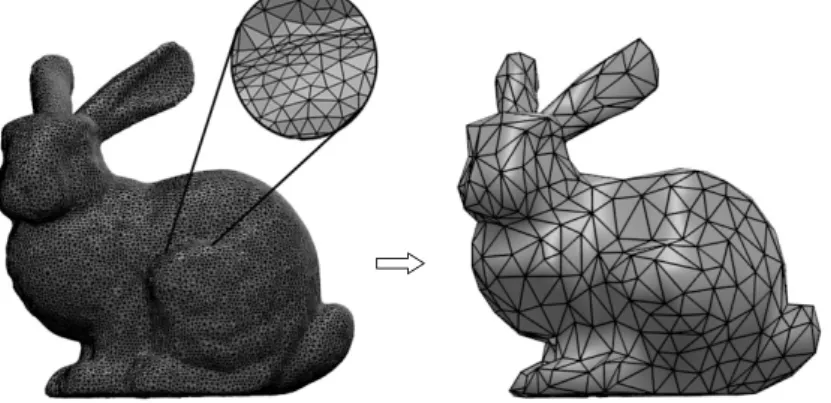
Figure 2: The original, detailed input mesh on the left and the simplified one on the right.
In the first optional step, the user can define the approximate number of the vertices of the cage. If it is equal to the number of vertices of the input, the step is skippable. Otherwise, the algorithm simplifies the input mesh using a decimation method (see Figure 2). We use the Quadric Edge Collapse Decimation method [5], but different ones can be used as well. Throughout the explanation of our algorithm, we refer this simplified mesh asinitial cage.
In the second step, the algorithm computes new vertex positions from the ones of the initial cage. The basic idea is the following: if a vertex of the initial cage is located in a high-curvature region of the surface, it will be positioned farther away from the surface than the others. Thus there is a higher chance to avoid the possible intersections.
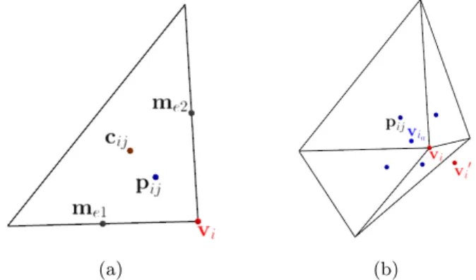
To compute the new position of the initial vertex vi ∈ V, at first, we have to define the face points pij of the connected faces at vertexvi by the following equation:
pij =me1+me2+cij+vi
4 , (4.1)
whereme1 andme2 are the midpoints of the edges that are adjacent to vertexvi, andcij is the center of the face (see Figure 3a).
After we have computed all face pointspij of the connected faces at vertexvi, we have to compute their averagevia calculated by the following equation:
via= 1 n
Xn
j=1
pij,
wherenis the number of faces which are connected at vertexvi.
Then, we can compute the new vertex positionv0i of the initial vertexvi (see Figure 3b) by the following equation:
v0i=vi+ d(vi,via)·n(vi),
wheren(vi)is the vertex normal atvi,||n(vi)||= 1, andd(vi,via)is the distance between verticesvi andvia.
(a) (b)
Figure 3: (a) A face and its face pointpij which is connected to vertexvi. (b) The new vertex positionvi0 which is computed from
the corresponding original vertex positionvi.
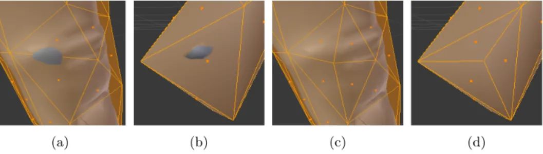
We notice that each face point pij can be considered as the barycentre of the polygon with vertices me1,me2,cij, andvi. If we define different weights w1, w2, w3, andw4 at the vertices of the polygon, we get distinct positions of the point on the face. Thus, we can adjust the distance between verticesviandvi0 (see Figure 4).
Thereby Equation 4.1 may be rewritten as follows:
pij =w1me1+w2me2+w3cij+w4vi, (4.2) wherew1+w2+w3+w4= 1.
After the second step has been completed, we get a cage mesh which envelops the input model. But intersections may still occur; thus, we remove them in the
(a) (b)
Figure 4: Face points are computed with different weights (a)wi=14,i∈ {1,2,3,4}, and (b)w1= 202,w2=202,w3 =1520 and w4 = 201. The distances between verticesvi andv0i are≈2.21(a)
and≈3.18(b).
last step of the algorithm. An edge or a face of the cage mesh can intersect the original model.
We correct both types of intersections locally but in different ways (see in Fig- ure 5). In the first case, we split both faces, which meet at the intersecting edge, into four new faces using a new vertex. To get this new vertex, we translate the average of the vertex positions of the mentioned original faces along its normal until the intersection disappears.
(a) (b) (c) (d)
Figure 5: An intersecting (a) edge and (b) face. (c) and (d) show the solutions to the intersection problems.
In the second case, when a face of the cage mesh intersects the original model, we split it into three new faces using a new vertex. We have to calculate the average of the vertex positions of the original intersecting face, then translate it along its normal until the intersection is disappeared.
In both cases, the algorithm works iteratively, therefore we can check that the intersection has already disappeared. The advantage of these solutions is that the error is eliminated locally by defining only one new vertex at a time and we will not yield other intersections in a neighbouring part. Furthermore, the positions of other vertices are not changed; thus, the distance between the cage and the original
mesh remains minimal. After all wrong edges and faces have been corrected, we get a cage mesh which envelops the original mesh without intersections.
4.1. Limitations
As we said, it cannot be proved that a cage can be generated for any input model with any number of cage faces. Therefore our algorithm will fail in some cases, like the previous works. Currently, it is an unsolved problem in the area.
The algorithm stops when the number of the steps required for correcting an intersection is greater than a user-specified limit. The same happens when the user defines a small number of cage vertices in the first step of the algorithm because the decimation method will result in a model with truncated limbs, therefore the second step can not be executed (see Figure 6).
Figure 6: An input model and a decimated mesh after the first simplification step. The decimation algorithm results in a model with truncated limbs because of the small number of cage vertices.
The workflow of our cage generation algorithm can be seen in Algorithm 1.
5. Results
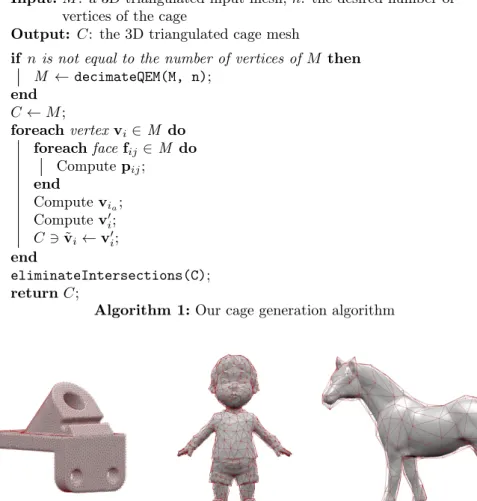
We tried our method on many meshes with different topologies from CAD models all the way up to animation characters (see Figure 7).
As we mentioned in Section 4, the first step of our algorithm is optional. If the user does not define the number of vertices of the cage mesh, the algorithm generates a cage which contains the same amount of vertices as the input model
Input:M: a 3D triangulated input mesh, n: the desired number of vertices of the cage
Output: C: the 3D triangulated cage mesh
if n is not equal to the number of vertices ofM then M ←decimateQEM(M, n);
end C←M;
foreachvertexvi∈M do foreachfacefij ∈M do
Computepij; endComputevia; Computev0i; C3v˜i←v0i;
endeliminateIntersections(C);
returnC;
Algorithm 1:Our cage generation algorithm
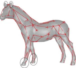
Figure 7: Input models and their generated cages in red. The user defined the desired number of the cage vertices.
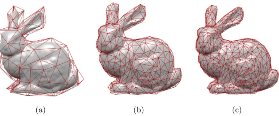
itself. But otherwise, the user may define the approximate number of vertices of the generated cage (see Figure 8).
We have shown previously in Section 4 that we can create cages for the same input model with different weights, so the distance between the input model and the cage is adjustable. Cage based deformation techniques have different important properties. One of them is that the reduction of the distance between the cage and the input model results in a much more efficient deformation. So, if we want to produce a sensitive deformation, we have to place equal weights at the vertices, but if we want to use a robust deformation, the least weight have to be placed at vertex vi, while the greatest at vertexcij (see Equation 4.2). This distance manipulation
(a) (b) (c) Figure 8: The Stanford Bunny as input model and the generated
cages with (a) 143, (b) 448, and (c) 805 vertices, respectively.
can be seen in Figure 9.
(a) (b)
Figure 9: Input model and generated cages with different weights (a)w1=w2=w3=w4= 14, and
(b)w1=w2 =1002 , w3= 10095 andw4= 1001 .
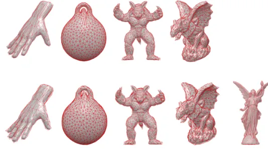
We compared our algorithm with the method of Sacht et al. [15]. We measured running times for comparing the algorithms on an Intel Core i7 4.4GHz processor with 16GB memory (see Table 1 and Figure 10). We can see that our algorithm was faster for every tested model, and the method of Sacht et al. failed in the case of model Angel Lucy.
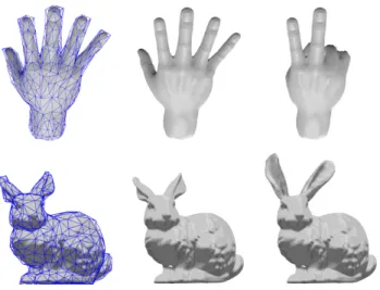
The constructed cage meshes are also usable for cage-based deformation tech- niques such as Mean Value Coordinates, Harmonic Coordinates, or Green Coordi- nates without modifications (see in Figure 11).
Model Input Faces Cage Faces Sacht et al.’s Our method
Hand 8808 600 16s 1s
Handles 47104 1500 30s 17s
Armadillo 12000 3000 35s 7s
Gargoyle 13500 2500 28.5s 6s
Angel Lucy 50000 10000 - 129s
Table 1: The comparison of the method of Sacht et al. and our algorithm. The last two columns show the running times in seconds.
Figure 10: The results of the method of Sacht et al. in the upper row. The outputs of our algorithm in the bottom row.
6. Future work
We plan to optimize the intersection detection step of the algorithm because it naively executes the search in each iteration step instead of updating.
The drawback of our algorithm is that it relies on the simplification of the input model. As we simplify the input model, the distance between the input and the resulting cage mesh is increased. Furthermore, under a certain number of cage vertices, our algorithm fails. Therefore, our future plan is to try different decimation algorithms [6, 11] which can preserve the topology of the input model, while the distance between the input and the resulting mesh remains minimal.
Figure 11: The figure shows the usage of our generated cages for model deformation.
Acknowledgements. The first author was supported by the construction EFOP- 3.6.3-VEKOP-16-2017-00002. The project was supported by the European Union, co-financed by the European Social Fund.
The second author was supported by the ÚNKP–17–4 New National Excel- lence Program Of The Ministry Of Human Capacities.
References
[1] Blanco, F. R. and Oliveira, M. M. (2008). Instant Mesh Deformation. InProceedings of the 2008 Symposium on Interactive 3D Graphics and Games, pages 71–78.
https://doi.org/10.1145/1342250.1342261
[2] Botsch, M. and Kobbelt, L. (2005). Real-Time Shape Editing using Radial Basis Functions. Computer Graphics Forum, 24(3):611–621.
https://doi.org/10.1111/j.1467-8659.2005.00886.x
[3] Deng, Z.-J., Luo, X.-N., and Miao, X.-P. (2011). Automatic Cage Building with Quadric Error Metrics. Journal of Computer Science and Technology, 26(3):538–
547.
https://doi.org/10.1007/s11390-011-1153-4
[4] Floater, M. S. (2015). Generalized barycentric coordinates and applications. Acta Numerica, 24:161–214.
https://doi.org/10.1017/S0962492914000129
[5] Garland, M. and Heckbert, P. S. (1997). Surface Simplification Using Quadric Error Metrics. In Proceedings of the 24th Annual Conference on Computer Graphics and Interactive Techniques, pages 209–216, New York, NY, USA. ACM Press/Addison-
Wesley Publishing Co.
https://doi.org/10.1145/258734.258849
[6] Gumhold, S., Borodin, P., and Klein, R. (2003). Intersection Free Simplification.
International Journal of Shape Modeling, 09(02):155–176.
https://doi.org/10.1142/S0218654303000097
[7] Jacobson, A., Baran, I., Popović, J., and Sorkine, O. (2011). Bounded Biharmonic Weights for Real-Time Deformation. ACM Transactions on Graphics, 30(4):78:1–
78:8.
https://doi.org/10.1145/2010324.1964973
[8] Joshi, P., Meyer, M., DeRose, T., Green, B., and Sanocki, T. (2007). Harmonic Coordinates for Character Articulation.ACM Transactions on Graphics, 26(3):71:1–
71:9, ISSN:0730-0301.
https://doi.org/10.1145/1276377.1276466
[9] Ju, T., Schaefer, S., and Warren, J. (2005). Mean Value Coordinates for Closed Tri- angular Meshes. ACM Transactions on Graphics, 24(3):561–566, ISSN:0730-0301.
https://doi.org/10.1145/1073204.1073229
[10] Le, B. H. and Deng, Z. (2017). Interactive Cage Generation for Mesh Deformation.
InProceedings of the 21st ACM SIGGRAPH Symposium on Interactive 3D Graphics and Games, pages 3:1–3:9, New York, NY, USA.
https://doi.org/10.1145/3023368.3023369
[11] Legrand, H. and Boubekeur, T. (2015). Morton Integrals for High Speed Geometry Simplification. InProceedings of the 7th Conference on High-Performance Graphics, HPG ’15, pages 105–112, New York, NY, USA.
https://doi.org/10.1145/2790060.2790071
[12] Lipman, Y., Levin, D., and Cohen-Or, D. (2008). Green Coordinates. ACM Trans- actions on Graphics, 27(3):78:1–78:10.
https://doi.org/10.1145/1360612.1360677
[13] Möbius, A. F. (1827). Der barycentrische Calcul. Johann Ambrosius Barth, Leipzig.
[14] Nieto, J. R. and Susín, A. (2013).Cage Based Deformations: A Survey, pages 75–99.
Springer Netherlands.
https://doi.org/10.1007/978-94-007-5446-1_3
[15] Sacht, L., Vouga, E., and Jacobson, A. (2015). Nested Cages.ACM Transactions on Graphics, 34(6):170:1–170:14.
https://doi.org/10.1145/2816795.2818093
[16] Sederberg, T. W. and Parry, S. R. (1986). Free-form Deformation of Solid Geometric Models. ACM SIGGRAPH Computer Graphics, 20(4):151–160.
https://doi.org/10.1145/15886.15903
[17] Sorkine, O. and Alexa, M. (2007). As-Rigid-As-Possible Surface Modeling. InPro- ceedings of the Fifth Eurographics Symposium on Geometry Processing, pages 109–
116. Eurographics Association.
[18] Xian, C., Lin, H., and Gao, S. (2012). Automatic cage generation by improved OBBs for mesh deformation. The Visual Computer, 28(1):21–33.
https://doi.org/10.1007/s00371-011-0595-6
[19] Yoshizawa, S., Belyaev, A., and Seidel, H.-P. (2007). Skeleton-based Variational Mesh Deformations. Computer Graphics Forum, 26(3):255–264.
https://doi.org/10.1111/j.1467-8659.2007.01047.x