Graph construction with condition-based weights for spectral clustering of hierarchical datasets
DOI: 10.36244/ICJ.2020.2.5
INFOCOMMUNICATIONS JOURNAL
Graph construction with condition-based weights for spectral clustering of hierarchical datasets
Dávid Papp1, Zsolt Knoll2, and Gábor Szűcs3
1,3Department of Telecommunications and Media Informatics, Budapest University of Technology and Economics, Budapest, Hungary; and Zs. Knoll (2) is student in BME Balatonfüred Student Research Group.
1,3E-mail: {pappd, szucs}@tmit.bme.hu
138 2
denote the similarity between 𝑥𝑥𝑖𝑖 and 𝑥𝑥𝑗𝑗 by 𝑠𝑠𝑖𝑖𝑗𝑗; classic spectral clustering method creates a similarity graph 𝐺𝐺, and then proceed as follows:
1. First, a similarity matrix 𝑆𝑆 is derived from 𝐺𝐺, where an 𝑠𝑠𝑖𝑖𝑗𝑗 element corresponds to the weight of the edge between 𝑥𝑥𝑖𝑖 and 𝑥𝑥𝑗𝑗 in 𝐺𝐺 (in case of not connected points 𝑠𝑠𝑖𝑖𝑗𝑗= 0).
2. Then diagonal matrix 𝐷𝐷 is calculated by summing the columns of 𝑆𝑆, as can be seen in Eq. 1.
𝐷𝐷 = {𝑑𝑑𝑖𝑖𝑖𝑖}; 𝑑𝑑𝑖𝑖𝑖𝑖= ∑ 𝑠𝑠𝑖𝑖𝑗𝑗 𝑗𝑗
(1) 3. After that the graph Laplacian matrix 𝐿𝐿 is
determined from 𝑆𝑆 and 𝐷𝐷 [12], which is a crucial part of spectral clustering, since different 𝐿𝐿 lead to different approach. In this paper the symmetric normalized graph Laplacian is used, which can be computed as expressed in Eq. 2.
𝐿𝐿𝑠𝑠𝑠𝑠𝑠𝑠= 𝐷𝐷−1 2⁄ ∗ 𝑆𝑆 ∗ 𝐷𝐷−1 2⁄ (2)
4. Calculate the first 𝑘𝑘 eigenvectors of 𝐿𝐿𝑠𝑠𝑠𝑠𝑠𝑠 and then construct a column matrix 𝑈𝑈 from these vectors.
5. Perform K-means clustering on the rows of 𝑈𝑈 to form 𝐶𝐶1, … , 𝐶𝐶𝑘𝑘.
Majority of authors use graph Laplacian matrix [3][26] in the spectral clustering method, but there is possibility to use other type, so called adjacency matrix [4][14][21]. The eigen decomposition step can be computationally intensive.
However, with an appropriate implementation, for example using sparse neighborhood graphs instead of all pairwise similarities, the memory and computational requirements can be solved. Several fast and approximate methods for spectral clustering have been proposed [6][17][28]. The traditional spectral clustering does not make any assumptions about the cluster shapes, but in our research, we dealt with point-sets instead of simple points, so points in a common set are expected to get a common cluster as well.
This concludes the spectral clustering and applying this procedure without any additional modification on a hierarchical dataset would result in a possible structure division. Two novel weight graphs were suggested, the Fully-Connected Weight Graph (FC-WG) and the Nearest Points of Point-sets Weight Graph (NPP-WG) [23]; that can influence the result of spectral clustering algorithms in such way that points belonging to the same point-set will stay together after the clustering is performed. To achieve this behavior the 𝐺𝐺 similarity graph in the original algorithm should be replaced with either FC-WG or NPP-WG. The former is a fully connected graph, where the
weight of an edge (𝑤𝑤𝑖𝑖𝑗𝑗) between two points (𝑥𝑥𝑖𝑖, 𝑥𝑥𝑗𝑗) is calculated according to Eq. 3. Basically the weight is higher in case 𝑥𝑥𝑖𝑖 and 𝑥𝑥𝑗𝑗 are part of the same point-set (xi↔ xj), and it is lower if they are not ( xi↮ xj).
𝑤𝑤𝑖𝑖𝑗𝑗= { 𝑛𝑛
𝑠𝑠𝑖𝑖𝑗𝑗 | xi↔ xj
xi↮ xj} (3)
where 𝑛𝑛 denotes the number of points in the dataset. The NPP-WG is an incomplete graph, because connections between different point-sets are limited, however points that are part of the same point-set still form a fully connected subgraph; as can be seen in Eq. 4.
𝑤𝑤𝑖𝑖𝑗𝑗= { 𝑛𝑛 sij
0 |
xi↔ xj
xi↮ xj & sij≥ sit: ∀𝑥𝑥𝑡𝑡 (xj↔ xt , 𝑥𝑥𝑗𝑗≠ 𝑥𝑥𝑡𝑡) 𝑜𝑜𝑜𝑜ℎ𝑒𝑒𝑒𝑒𝑤𝑤𝑒𝑒𝑠𝑠𝑒𝑒
} (4) The fundamental idea behind these modifications is to connect any two points inside the same point-set with an increased edge weight that is higher than 𝑠𝑠𝑖𝑖𝑗𝑗. Although this adjustment does not guarantee that the point-sets remain intact, it only reduces the chance to separate them. The focus of our research was to establish a set of conditions that the weighted graph creation process should satisfy in order to ensure the preservation of point-sets in the hierarchical dataset. In the next section we present the proposed condition system, then Section III contains the result of our experimental evaluation, and in the last section the conclusions of the research are summarized.
II. SET OF CONDITIONS FOR WEIGHTED GRAPH CONSTRUCTION With appropriate conditions can be achieved that the points in the same point-set stay together, when using FC-WG and NPP-WG methods. For the formulas the following notations were used:
𝑛𝑛: 𝑛𝑛𝑛𝑛𝑛𝑛𝑛𝑛𝑒𝑒𝑒𝑒 𝑜𝑜𝑜𝑜 𝑝𝑝𝑜𝑜𝑒𝑒𝑛𝑛𝑜𝑜𝑠𝑠 𝑘𝑘: 𝑛𝑛𝑛𝑛𝑛𝑛𝑛𝑛𝑒𝑒𝑒𝑒 𝑜𝑜𝑜𝑜 𝑐𝑐𝑐𝑐𝑛𝑛𝑠𝑠𝑜𝑜𝑒𝑒𝑒𝑒𝑠𝑠 𝐶𝐶𝑖𝑖: 𝑒𝑒𝑡𝑡ℎ 𝑐𝑐𝑐𝑐𝑛𝑛𝑠𝑠𝑜𝑜𝑒𝑒𝑒𝑒
|𝐶𝐶𝑖𝑖|: 𝑛𝑛𝑛𝑛𝑛𝑛𝑛𝑛𝑒𝑒𝑒𝑒 𝑜𝑜𝑜𝑜 𝑑𝑑𝑑𝑑𝑜𝑜𝑑𝑑𝑝𝑝𝑜𝑜𝑒𝑒𝑛𝑛𝑜𝑜𝑠𝑠 𝑒𝑒𝑛𝑛 𝑜𝑜ℎ𝑒𝑒 𝑒𝑒𝑡𝑡ℎ 𝑐𝑐𝑐𝑐𝑛𝑛𝑠𝑠𝑜𝑜𝑒𝑒𝑒𝑒 𝐶𝐶̅: 𝑐𝑐𝑜𝑜𝑛𝑛𝑝𝑝𝑐𝑐𝑒𝑒𝑛𝑛𝑒𝑒𝑛𝑛𝑜𝑜 𝑜𝑜𝑜𝑜 𝐶𝐶𝑖𝑖 𝑖𝑖
𝑆𝑆𝑖𝑖: 𝑒𝑒𝑡𝑡ℎ 𝑝𝑝𝑜𝑜𝑒𝑒𝑛𝑛𝑜𝑜𝑠𝑠𝑒𝑒𝑜𝑜 𝐴𝐴: 𝑠𝑠𝑒𝑒𝑛𝑛𝑒𝑒𝑐𝑐𝑑𝑑𝑒𝑒𝑒𝑒𝑜𝑜𝑠𝑠 𝑛𝑛𝑑𝑑𝑜𝑜𝑒𝑒𝑒𝑒𝑥𝑥
𝐴𝐴𝑖𝑖𝑗𝑗: 𝑜𝑜ℎ𝑒𝑒 𝑗𝑗𝑡𝑡ℎ𝑒𝑒𝑐𝑐𝑒𝑒𝑛𝑛𝑒𝑒𝑛𝑛𝑜𝑜 𝑜𝑜𝑜𝑜 𝑜𝑜ℎ𝑒𝑒 𝑒𝑒𝑡𝑡ℎ 𝑒𝑒𝑜𝑜𝑤𝑤 𝑒𝑒𝑛𝑛 𝑜𝑜ℎ𝑒𝑒 𝐴𝐴 𝑛𝑛𝑑𝑑𝑜𝑜𝑒𝑒𝑒𝑒𝑥𝑥 𝑍𝑍: 𝑒𝑒𝑑𝑑𝑒𝑒𝑒𝑒 𝑤𝑤𝑒𝑒𝑒𝑒𝑒𝑒𝑜𝑜ℎ𝑠𝑠 𝑒𝑒𝑛𝑛𝑠𝑠𝑒𝑒𝑑𝑑𝑒𝑒 𝑝𝑝𝑜𝑜𝑒𝑒𝑛𝑛𝑜𝑜 𝑠𝑠𝑒𝑒𝑜𝑜𝑠𝑠
The normalized spectral clustering is the relaxation of the normalized cut [26][27]:
𝑁𝑁𝑐𝑐𝑛𝑛𝑜𝑜(𝐶𝐶1, … , 𝐶𝐶𝑘𝑘) = ∑𝑐𝑐𝑛𝑛𝑜𝑜(𝐶𝐶𝑖𝑖, 𝐶𝐶̅)𝑖𝑖
𝑣𝑣𝑜𝑜𝑐𝑐(𝐶𝐶𝑖𝑖)
𝑘𝑘 𝑖𝑖=1
=
=1
2 ∑
∑𝑗𝑗∈𝐶𝐶𝑖𝑖∑𝑗𝑗∈𝐶𝐶̅𝑖𝑖𝐴𝐴𝑗𝑗𝑗𝑗
∑𝑗𝑗∈𝐶𝐶𝑖𝑖∑𝑗𝑗∈𝐶𝐶̅𝑖𝑖𝐴𝐴𝑗𝑗𝑗𝑗+ ∑𝑗𝑗∈𝐶𝐶𝑖𝑖∑𝑗𝑗∈𝐶𝐶𝑖𝑖𝐴𝐴𝑗𝑗𝑗𝑗 𝑘𝑘
𝑖𝑖=1
(5)
138 1
Abstract—Most of the unsupervised machine learning algorithms focus on clustering the data based on similarity metrics, while ignoring other attributes, or perhaps other type of connections between the data points. In case of hierarchical datasets, groups of points (point-sets) can be defined according to the hierarchy system. Our goal was to develop such spectral clustering approach that preserves the structure of the dataset throughout the clustering procedure. The main contribution of this paper is a set of conditions for weighted graph construction used in spectral clustering. Following the requirements – given by the set of conditions – ensures that the hierarchical formation of the dataset remains unchanged, and therefore the clustering of data points imply the clustering of point-sets as well. The proposed spectral clustering algorithm was tested on three datasets, the results were compared to baseline methods and it can be concluded the algorithm with the proposed conditions always preserves the hierarchy structure.
Index Terms—spectral clustering, hierarchical dataset, graph construction
I. INTRODUCTION
Many clustering methods have been developed, each of which uses a different induction principle [22][29]. Farley and Raftery [8] suggest dividing the clustering methods into two main groups: hierarchical and partitioning methods [25]; and other authors [10] suggest categorizing the methods into additional three main categories: density-based methods [5], model-based clustering [19] and grid-based methods [11].
Partitioning methods are divided into two groups: center-based and graph-theoretic clustering (spectral clustering).
Clusterability for spectral clustering, i.e. the problem of defining what is a “good” clustering, has been studied in some papers [1][2]. HSC [16] algorithm was developed to cluster arbitrarily shaped data more efficiently and accurately by combining spectral and hierarchical clustering techniques.
Francky Fouedjio suggested a novel spectral clustering algorithm, which integrates such similarity measure that takes into account the spatial dependency of data, and therefore it is able to discover spatially contiguous and meaningful clusters in multivariate geostatistical data [9]. Furthermore, Li and Huang proposed an effective hierarchical clustering algorithm called D. Papp and G. Szűcs are with the Department of Telecommunications and Media Informatics, Budapest University of Technology and Economics,
SHC [15] that is based on the techniques of spectral clustering method. Although, none of the above studies focus on the case when the input dataset itself is a hierarchical dataset. The spectral clustering method is computationally expensive compared to e.g. center-based clustering, as it needs to store and manipulate similarities (or distances) between all pairs of points instead of only distances to centers [20].
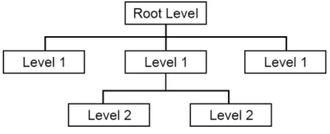
A regular dataset 𝑋𝑋 = {𝑥𝑥1, … , 𝑥𝑥𝑛𝑛} consists of 𝑛𝑛 data points and usually there is no pre-defined connection between any two (𝑥𝑥𝑖𝑖, 𝑥𝑥𝑗𝑗) data points. Then clustering 𝑋𝑋 into 𝑘𝑘 clusters can be performed without any restriction on the composition of clusters; this process yields clusters 𝐶𝐶1, … , 𝐶𝐶𝑘𝑘. On the other hand, a hierarchical dataset designates parent-child relationships between the points (as can be seen in Fig. 1); e.g.
𝑥𝑥𝑖𝑖 and 𝑥𝑥𝑗𝑗 could be the children of 𝑥𝑥𝑙𝑙, so in this case (𝑥𝑥𝑖𝑖, 𝑥𝑥𝑗𝑗) together form a so called point-set.
Figure 1. Structure of hierarchical dataset
Performing a traditional clustering algorithm also produces the 𝐶𝐶1, … , 𝐶𝐶𝑘𝑘 clusters, however 𝑥𝑥𝑖𝑖 could be part of 𝐶𝐶𝑔𝑔, while 𝑥𝑥𝑗𝑗
could be assigned to 𝐶𝐶ℎ, and therefore the (𝑥𝑥𝑖𝑖, 𝑥𝑥𝑗𝑗) point-set would be separated. This means that it is possible that clustering breaks the hierarchical structure of the dataset. In this paper we propose a set of conditions to control the weighted graph creation procedure in the course of spectral clustering [27]
algorithm. Using the graph built accordingly will prevent the splitting of point-sets during clustering.
There are several different techniques to build the similarity graph in the spectral clustering, e.g. the ε-neighborhood, k- nearest neighbor and fully connected graphs [27]. The difference between them is how they determine whether two vertices (𝑥𝑥𝑖𝑖 and 𝑥𝑥𝑗𝑗) are connected by an edge or not. Let us Hungary; and Zs. Knoll is student in the same university. (e-mail:
pappd@tmit.bme.hu, szucs@tmit.bme.hu)
Graph construction with condition-based weights for spectral clustering of hierarchical datasets
Dávid Papp, Zsolt Knoll, Gábor Szűcs
138 1
Abstract—Most of the unsupervised machine learning algorithms focus on clustering the data based on similarity metrics, while ignoring other attributes, or perhaps other type of connections between the data points. In case of hierarchical datasets, groups of points (point-sets) can be defined according to the hierarchy system. Our goal was to develop such spectral clustering approach that preserves the structure of the dataset throughout the clustering procedure. The main contribution of this paper is a set of conditions for weighted graph construction used in spectral clustering. Following the requirements – given by the set of conditions – ensures that the hierarchical formation of the dataset remains unchanged, and therefore the clustering of data points imply the clustering of point-sets as well. The proposed spectral clustering algorithm was tested on three datasets, the results were compared to baseline methods and it can be concluded the algorithm with the proposed conditions always preserves the hierarchy structure.
Index Terms—spectral clustering, hierarchical dataset, graph construction
I. INTRODUCTION
Many clustering methods have been developed, each of which uses a different induction principle [22][29]. Farley and Raftery [8] suggest dividing the clustering methods into two main groups: hierarchical and partitioning methods [25]; and other authors [10] suggest categorizing the methods into additional three main categories: density-based methods [5], model-based clustering [19] and grid-based methods [11].
Partitioning methods are divided into two groups: center-based and graph-theoretic clustering (spectral clustering).
Clusterability for spectral clustering, i.e. the problem of defining what is a “good” clustering, has been studied in some papers [1][2]. HSC [16] algorithm was developed to cluster arbitrarily shaped data more efficiently and accurately by combining spectral and hierarchical clustering techniques.
Francky Fouedjio suggested a novel spectral clustering algorithm, which integrates such similarity measure that takes into account the spatial dependency of data, and therefore it is able to discover spatially contiguous and meaningful clusters in multivariate geostatistical data [9]. Furthermore, Li and Huang proposed an effective hierarchical clustering algorithm called D. Papp and G. Szűcs are with the Department of Telecommunications and Media Informatics, Budapest University of Technology and Economics,
SHC [15] that is based on the techniques of spectral clustering method. Although, none of the above studies focus on the case when the input dataset itself is a hierarchical dataset. The spectral clustering method is computationally expensive compared to e.g. center-based clustering, as it needs to store and manipulate similarities (or distances) between all pairs of points instead of only distances to centers [20].
A regular dataset 𝑋𝑋 = {𝑥𝑥1, … , 𝑥𝑥𝑛𝑛} consists of 𝑛𝑛 data points and usually there is no pre-defined connection between any two (𝑥𝑥𝑖𝑖, 𝑥𝑥𝑗𝑗) data points. Then clustering 𝑋𝑋 into 𝑘𝑘 clusters can be performed without any restriction on the composition of clusters; this process yields clusters 𝐶𝐶1, … , 𝐶𝐶𝑘𝑘. On the other hand, a hierarchical dataset designates parent-child relationships between the points (as can be seen in Fig. 1); e.g.
𝑥𝑥𝑖𝑖 and 𝑥𝑥𝑗𝑗 could be the children of 𝑥𝑥𝑙𝑙, so in this case (𝑥𝑥𝑖𝑖, 𝑥𝑥𝑗𝑗) together form a so called point-set.
Figure 1. Structure of hierarchical dataset
Performing a traditional clustering algorithm also produces the 𝐶𝐶1, … , 𝐶𝐶𝑘𝑘 clusters, however 𝑥𝑥𝑖𝑖 could be part of 𝐶𝐶𝑔𝑔, while 𝑥𝑥𝑗𝑗
could be assigned to 𝐶𝐶ℎ, and therefore the (𝑥𝑥𝑖𝑖, 𝑥𝑥𝑗𝑗) point-set would be separated. This means that it is possible that clustering breaks the hierarchical structure of the dataset. In this paper we propose a set of conditions to control the weighted graph creation procedure in the course of spectral clustering [27]
algorithm. Using the graph built accordingly will prevent the splitting of point-sets during clustering.
There are several different techniques to build the similarity graph in the spectral clustering, e.g. the ε-neighborhood, k- nearest neighbor and fully connected graphs [27]. The difference between them is how they determine whether two vertices (𝑥𝑥𝑖𝑖 and 𝑥𝑥𝑗𝑗) are connected by an edge or not. Let us Hungary; and Zs. Knoll is student in the same university. (e-mail:
pappd@tmit.bme.hu, szucs@tmit.bme.hu)
Graph construction with condition-based weights for spectral clustering of hierarchical datasets
Dávid Papp, Zsolt Knoll, Gábor Szűcs
denote the similarity between 𝑥𝑥𝑖𝑖 and 𝑥𝑥𝑗𝑗 by 𝑠𝑠𝑖𝑖𝑗𝑗; classic spectral clustering method creates a similarity graph 𝐺𝐺, and then proceed as follows:
1. First, a similarity matrix 𝑆𝑆 is derived from 𝐺𝐺, where an 𝑠𝑠𝑖𝑖𝑗𝑗 element corresponds to the weight of the edge between 𝑥𝑥𝑖𝑖 and 𝑥𝑥𝑗𝑗 in 𝐺𝐺 (in case of not connected points 𝑠𝑠𝑖𝑖𝑗𝑗= 0).
2. Then diagonal matrix 𝐷𝐷 is calculated by summing the columns of 𝑆𝑆, as can be seen in Eq. 1.
𝐷𝐷 = {𝑑𝑑𝑖𝑖𝑖𝑖}; 𝑑𝑑𝑖𝑖𝑖𝑖= ∑ 𝑠𝑠𝑖𝑖𝑗𝑗 𝑗𝑗
(1) 3. After that the graph Laplacian matrix 𝐿𝐿 is
determined from 𝑆𝑆 and 𝐷𝐷 [12], which is a crucial part of spectral clustering, since different 𝐿𝐿 lead to different approach. In this paper the symmetric normalized graph Laplacian is used, which can be computed as expressed in Eq. 2.
𝐿𝐿𝑠𝑠𝑠𝑠𝑠𝑠= 𝐷𝐷−1 2⁄ ∗ 𝑆𝑆 ∗ 𝐷𝐷−1 2⁄ (2)
4. Calculate the first 𝑘𝑘 eigenvectors of 𝐿𝐿𝑠𝑠𝑠𝑠𝑠𝑠 and then construct a column matrix 𝑈𝑈 from these vectors.
5. Perform K-means clustering on the rows of 𝑈𝑈 to form 𝐶𝐶1, … , 𝐶𝐶𝑘𝑘.
Majority of authors use graph Laplacian matrix [3][26] in the spectral clustering method, but there is possibility to use other type, so called adjacency matrix [4][14][21]. The eigen decomposition step can be computationally intensive.
However, with an appropriate implementation, for example using sparse neighborhood graphs instead of all pairwise similarities, the memory and computational requirements can be solved. Several fast and approximate methods for spectral clustering have been proposed [6][17][28]. The traditional spectral clustering does not make any assumptions about the cluster shapes, but in our research, we dealt with point-sets instead of simple points, so points in a common set are expected to get a common cluster as well.
This concludes the spectral clustering and applying this procedure without any additional modification on a hierarchical dataset would result in a possible structure division. Two novel weight graphs were suggested, the Fully-Connected Weight Graph (FC-WG) and the Nearest Points of Point-sets Weight Graph (NPP-WG) [23]; that can influence the result of spectral clustering algorithms in such way that points belonging to the same point-set will stay together after the clustering is performed. To achieve this behavior the 𝐺𝐺 similarity graph in the original algorithm should be replaced with either FC-WG or NPP-WG. The former is a fully connected graph, where the
weight of an edge (𝑤𝑤𝑖𝑖𝑗𝑗) between two points (𝑥𝑥𝑖𝑖, 𝑥𝑥𝑗𝑗) is calculated according to Eq. 3. Basically the weight is higher in case 𝑥𝑥𝑖𝑖 and 𝑥𝑥𝑗𝑗 are part of the same point-set (xi↔ xj), and it is lower if they are not ( xi↮ xj).
𝑤𝑤𝑖𝑖𝑗𝑗= { 𝑛𝑛
𝑠𝑠𝑖𝑖𝑗𝑗 | xi↔ xj
xi↮ xj} (3)
where 𝑛𝑛 denotes the number of points in the dataset. The NPP-WG is an incomplete graph, because connections between different point-sets are limited, however points that are part of the same point-set still form a fully connected subgraph; as can be seen in Eq. 4.
𝑤𝑤𝑖𝑖𝑗𝑗= { 𝑛𝑛 sij
0 |
xi↔ xj
xi↮ xj & sij≥ sit: ∀𝑥𝑥𝑡𝑡 (xj↔ xt , 𝑥𝑥𝑗𝑗≠ 𝑥𝑥𝑡𝑡) 𝑜𝑜𝑜𝑜ℎ𝑒𝑒𝑒𝑒𝑤𝑤𝑒𝑒𝑠𝑠𝑒𝑒
} (4) The fundamental idea behind these modifications is to connect any two points inside the same point-set with an increased edge weight that is higher than 𝑠𝑠𝑖𝑖𝑗𝑗. Although this adjustment does not guarantee that the point-sets remain intact, it only reduces the chance to separate them. The focus of our research was to establish a set of conditions that the weighted graph creation process should satisfy in order to ensure the preservation of point-sets in the hierarchical dataset. In the next section we present the proposed condition system, then Section III contains the result of our experimental evaluation, and in the last section the conclusions of the research are summarized.
II. SET OF CONDITIONS FOR WEIGHTED GRAPH CONSTRUCTION With appropriate conditions can be achieved that the points in the same point-set stay together, when using FC-WG and NPP-WG methods. For the formulas the following notations were used:
𝑛𝑛: 𝑛𝑛𝑛𝑛𝑛𝑛𝑛𝑛𝑒𝑒𝑒𝑒 𝑜𝑜𝑜𝑜 𝑝𝑝𝑜𝑜𝑒𝑒𝑛𝑛𝑜𝑜𝑠𝑠 𝑘𝑘: 𝑛𝑛𝑛𝑛𝑛𝑛𝑛𝑛𝑒𝑒𝑒𝑒 𝑜𝑜𝑜𝑜 𝑐𝑐𝑐𝑐𝑛𝑛𝑠𝑠𝑜𝑜𝑒𝑒𝑒𝑒𝑠𝑠 𝐶𝐶𝑖𝑖: 𝑒𝑒𝑡𝑡ℎ 𝑐𝑐𝑐𝑐𝑛𝑛𝑠𝑠𝑜𝑜𝑒𝑒𝑒𝑒
|𝐶𝐶𝑖𝑖|: 𝑛𝑛𝑛𝑛𝑛𝑛𝑛𝑛𝑒𝑒𝑒𝑒 𝑜𝑜𝑜𝑜 𝑑𝑑𝑑𝑑𝑜𝑜𝑑𝑑𝑝𝑝𝑜𝑜𝑒𝑒𝑛𝑛𝑜𝑜𝑠𝑠 𝑒𝑒𝑛𝑛 𝑜𝑜ℎ𝑒𝑒 𝑒𝑒𝑡𝑡ℎ 𝑐𝑐𝑐𝑐𝑛𝑛𝑠𝑠𝑜𝑜𝑒𝑒𝑒𝑒 𝐶𝐶̅: 𝑐𝑐𝑜𝑜𝑛𝑛𝑝𝑝𝑐𝑐𝑒𝑒𝑛𝑛𝑒𝑒𝑛𝑛𝑜𝑜 𝑜𝑜𝑜𝑜 𝐶𝐶𝑖𝑖 𝑖𝑖
𝑆𝑆𝑖𝑖: 𝑒𝑒𝑡𝑡ℎ 𝑝𝑝𝑜𝑜𝑒𝑒𝑛𝑛𝑜𝑜𝑠𝑠𝑒𝑒𝑜𝑜 𝐴𝐴: 𝑠𝑠𝑒𝑒𝑛𝑛𝑒𝑒𝑐𝑐𝑑𝑑𝑒𝑒𝑒𝑒𝑜𝑜𝑠𝑠 𝑛𝑛𝑑𝑑𝑜𝑜𝑒𝑒𝑒𝑒𝑥𝑥
𝐴𝐴𝑖𝑖𝑗𝑗: 𝑜𝑜ℎ𝑒𝑒 𝑗𝑗𝑡𝑡ℎ𝑒𝑒𝑐𝑐𝑒𝑒𝑛𝑛𝑒𝑒𝑛𝑛𝑜𝑜 𝑜𝑜𝑜𝑜 𝑜𝑜ℎ𝑒𝑒 𝑒𝑒𝑡𝑡ℎ 𝑒𝑒𝑜𝑜𝑤𝑤 𝑒𝑒𝑛𝑛 𝑜𝑜ℎ𝑒𝑒 𝐴𝐴 𝑛𝑛𝑑𝑑𝑜𝑜𝑒𝑒𝑒𝑒𝑥𝑥 𝑍𝑍: 𝑒𝑒𝑑𝑑𝑒𝑒𝑒𝑒 𝑤𝑤𝑒𝑒𝑒𝑒𝑒𝑒𝑜𝑜ℎ𝑠𝑠 𝑒𝑒𝑛𝑛𝑠𝑠𝑒𝑒𝑑𝑑𝑒𝑒 𝑝𝑝𝑜𝑜𝑒𝑒𝑛𝑛𝑜𝑜 𝑠𝑠𝑒𝑒𝑜𝑜𝑠𝑠
The normalized spectral clustering is the relaxation of the normalized cut [26][27]:
𝑁𝑁𝑐𝑐𝑛𝑛𝑜𝑜(𝐶𝐶1, … , 𝐶𝐶𝑘𝑘) = ∑𝑐𝑐𝑛𝑛𝑜𝑜(𝐶𝐶𝑖𝑖, 𝐶𝐶̅)𝑖𝑖
𝑣𝑣𝑜𝑜𝑐𝑐(𝐶𝐶𝑖𝑖)
𝑘𝑘 𝑖𝑖=1
=
=1
2 ∑
∑𝑗𝑗∈𝐶𝐶𝑖𝑖∑𝑗𝑗∈𝐶𝐶̅𝑖𝑖𝐴𝐴𝑗𝑗𝑗𝑗
∑𝑗𝑗∈𝐶𝐶𝑖𝑖∑𝑗𝑗∈𝐶𝐶̅𝑖𝑖𝐴𝐴𝑗𝑗𝑗𝑗+ ∑𝑗𝑗∈𝐶𝐶𝑖𝑖∑𝑗𝑗∈𝐶𝐶𝑖𝑖𝐴𝐴𝑗𝑗𝑗𝑗 𝑘𝑘
𝑖𝑖=1
(5)
Abstract—Most of the unsupervised machine learning algorithms focus on clustering the data based on similarity metrics, while ignoring other attributes, or perhaps other type of connections between the data points. In case of hierarchical datasets, groups of points (point-sets) can be defined according to the hierarchy system. Our goal was to develop such spectral clustering approach that preserves the structure of the dataset throughout the clustering procedure. The main contribution of this paper is a set of conditions for weighted graph construction used in spectral clustering. Following the requirements – given by the set of conditions – ensures that the hierarchical formation of the dataset remains unchanged, and therefore the clustering of data points imply the clustering of point-sets as well. The proposed spectral clustering algorithm was tested on three datasets, the results were compared to baseline methods and it can be concluded the algorithm with the proposed conditions always preserves the hierarchy structure.
Index Terms—spectral clustering, hierarchical dataset, graph construction
I. INTRODUCTION
Many clustering methods have been developed, each of which uses a different induction principle [22][29]. Farley and Raftery [8] suggest dividing the clustering methods into two main groups: hierarchical and partitioning methods [25]; and other authors [10] suggest categorizing the methods into additional three main categories: density-based methods [5], model-based clustering [19] and grid-based methods [11].
Partitioning methods are divided into two groups: center-based and graph-theoretic clustering (spectral clustering).
Clusterability for spectral clustering, i.e. the problem of defining what is a “good” clustering, has been studied in some papers [1][2]. HSC [16] algorithm was developed to cluster arbitrarily shaped data more efficiently and accurately by combining spectral and hierarchical clustering techniques.
Francky Fouedjio suggested a novel spectral clustering algorithm, which integrates such similarity measure that takes into account the spatial dependency of data, and therefore it is able to discover spatially contiguous and meaningful clusters in multivariate geostatistical data [9]. Furthermore, Li and Huang proposed an effective hierarchical clustering algorithm called D. Papp and G. Szűcs are with the Department of Telecommunications and Media Informatics, Budapest University of Technology and Economics,
SHC [15] that is based on the techniques of spectral clustering method. Although, none of the above studies focus on the case when the input dataset itself is a hierarchical dataset. The spectral clustering method is computationally expensive compared to e.g. center-based clustering, as it needs to store and manipulate similarities (or distances) between all pairs of points instead of only distances to centers [20].
A regular dataset 𝑋𝑋 = {𝑥𝑥1, … , 𝑥𝑥𝑛𝑛} consists of 𝑛𝑛 data points and usually there is no pre-defined connection between any two (𝑥𝑥𝑖𝑖, 𝑥𝑥𝑗𝑗) data points. Then clustering 𝑋𝑋 into 𝑘𝑘 clusters can be performed without any restriction on the composition of clusters; this process yields clusters 𝐶𝐶1, … , 𝐶𝐶𝑘𝑘. On the other hand, a hierarchical dataset designates parent-child relationships between the points (as can be seen in Fig. 1); e.g.
𝑥𝑥𝑖𝑖 and 𝑥𝑥𝑗𝑗 could be the children of 𝑥𝑥𝑙𝑙, so in this case (𝑥𝑥𝑖𝑖, 𝑥𝑥𝑗𝑗) together form a so called point-set.
Figure 1. Structure of hierarchical dataset
Performing a traditional clustering algorithm also produces the 𝐶𝐶1, … , 𝐶𝐶𝑘𝑘 clusters, however 𝑥𝑥𝑖𝑖 could be part of 𝐶𝐶𝑔𝑔, while 𝑥𝑥𝑗𝑗
could be assigned to 𝐶𝐶ℎ, and therefore the (𝑥𝑥𝑖𝑖, 𝑥𝑥𝑗𝑗) point-set would be separated. This means that it is possible that clustering breaks the hierarchical structure of the dataset. In this paper we propose a set of conditions to control the weighted graph creation procedure in the course of spectral clustering [27]
algorithm. Using the graph built accordingly will prevent the splitting of point-sets during clustering.
There are several different techniques to build the similarity graph in the spectral clustering, e.g. the ε-neighborhood, k- nearest neighbor and fully connected graphs [27]. The difference between them is how they determine whether two vertices (𝑥𝑥𝑖𝑖 and 𝑥𝑥𝑗𝑗) are connected by an edge or not. Let us Hungary; and Zs. Knoll is student in the same university. (e-mail:
pappd@tmit.bme.hu, szucs@tmit.bme.hu)
Graph construction with condition-based weights for spectral clustering of hierarchical datasets
Dávid Papp, Zsolt Knoll, Gábor Szűcs
138 4
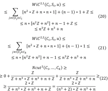
𝑊𝑊𝑊𝑊𝑊𝑊2,1(𝑊𝑊𝑖𝑖, 𝑆𝑆𝑡𝑡, 𝑢𝑢) ≤
≤ ∑ [𝑛𝑛2∗ 𝑍𝑍 + 𝑛𝑛 ∗ 𝑛𝑛 ∗ 1]
𝑗𝑗≠𝑡𝑡|𝑆𝑆𝑗𝑗∈𝐶𝐶𝑖𝑖
+ (𝑛𝑛 − 1) ∗ 1 + 𝑍𝑍 ≤
≤ 𝑛𝑛 ∗ [𝑛𝑛2𝑍𝑍 + 𝑛𝑛2] + 𝑛𝑛 − 1 + 𝑍𝑍 ≤
≤ 𝑛𝑛3𝑍𝑍 + 𝑛𝑛3+ 𝑛𝑛
(20)
𝑊𝑊𝑊𝑊𝑊𝑊2,2(𝑊𝑊𝑖𝑖, 𝑆𝑆𝑡𝑡, 𝑢𝑢) ≤
≤ ∑ [𝑛𝑛2∗ 𝑍𝑍 + 𝑛𝑛 ∗ 𝑛𝑛 ∗ 1]
𝑗𝑗≠𝑡𝑡|𝑆𝑆𝑗𝑗∈𝐶𝐶𝑘𝑘
+ (𝑛𝑛 − 1) ∗ 1 ≤
≤ 𝑛𝑛 ∗ [𝑛𝑛2𝑍𝑍 + 𝑛𝑛2] + 𝑛𝑛 − 1 ≤ 𝑛𝑛3𝑍𝑍 + 𝑛𝑛3+ 𝑛𝑛
(21)
𝑁𝑁𝑁𝑁𝑢𝑢𝑁𝑁2(𝑊𝑊1, … , 𝑊𝑊𝑘𝑘) ≥
≥ 0 + 𝑍𝑍
𝑍𝑍 + 𝑛𝑛3∗ 𝑍𝑍 + 𝑛𝑛3+ 𝑛𝑛 + 𝑍𝑍 +
𝑍𝑍
𝑍𝑍 + 𝑛𝑛3∗ 𝑍𝑍 + 𝑛𝑛3+ 𝑛𝑛 ≥
≥ 2 ∗ 𝑍𝑍
𝑍𝑍 + 𝑛𝑛3∗ 𝑍𝑍 + 𝑛𝑛3+ 𝑛𝑛 + 𝑍𝑍 =
2 ∗ 𝑍𝑍 (𝑛𝑛3+ 2) ∗ 𝑍𝑍 + 𝑛𝑛3+ 𝑛𝑛
(22)
The value of 𝑁𝑁𝑁𝑁𝑢𝑢𝑁𝑁1 should be lower than 𝑁𝑁𝑁𝑁𝑢𝑢𝑁𝑁2 in every case. Furthermore, both of them contain a multiplier of ½, and thus it could be eliminated in the equations.
𝑁𝑁𝑁𝑁𝑢𝑢𝑁𝑁1(𝑊𝑊1, … , 𝑊𝑊𝑘𝑘) < 𝑁𝑁𝑁𝑁𝑢𝑢𝑁𝑁2(𝑊𝑊1, … , 𝑊𝑊𝑘𝑘) (23) 𝑘𝑘 ∗ 𝑛𝑛
𝑛𝑛 + 𝑍𝑍< 2 ∗ 𝑍𝑍
(𝑛𝑛3+ 2) ∗ 𝑍𝑍 + 𝑛𝑛3+ 𝑛𝑛 (24) 0 < 2𝑍𝑍2+ (2𝑛𝑛 − 𝑘𝑘𝑛𝑛4− 2𝑘𝑘𝑛𝑛)𝑍𝑍 − (𝑘𝑘𝑛𝑛4+ 𝑘𝑘𝑛𝑛2) (25) 𝑌𝑌 = √𝑘𝑘2𝑛𝑛8+ 4𝑘𝑘2𝑛𝑛5+ 4𝑘𝑘2𝑛𝑛2+ 8𝑘𝑘𝑛𝑛4− 4𝑘𝑘𝑛𝑛5+ 4𝑛𝑛2 (26)
𝑍𝑍 <𝑘𝑘𝑛𝑛4+ 2𝑘𝑘𝑛𝑛 − 2𝑛𝑛 − 𝑌𝑌
4 (27)
or
𝑍𝑍 >𝑘𝑘𝑛𝑛4+ 2𝑘𝑘𝑛𝑛 − 2𝑛𝑛 + 𝑌𝑌
4 (28)
Both (27) and (28) fulfills the conditions in (24) and (25), but the value of (27) is negative in all cases (see Eq. 29, 30 and 31), which means that (27) can not be interpreted as a similarity value.
𝑘𝑘𝑛𝑛4+ 2𝑘𝑘𝑛𝑛 − 2𝑛𝑛 − 𝑌𝑌 < 0 (29) 𝑘𝑘2𝑛𝑛8+ 4𝑘𝑘2𝑛𝑛2+ 4𝑛𝑛2+ 4𝑘𝑘2𝑛𝑛5− 4𝑘𝑘𝑛𝑛5− 8𝑘𝑘𝑛𝑛2<
< 𝑘𝑘2𝑛𝑛8+ 4𝑘𝑘2𝑛𝑛5+ 4𝑘𝑘2𝑛𝑛2+ 8𝑘𝑘𝑛𝑛4− 4𝑘𝑘𝑛𝑛5+ 4𝑛𝑛2 (30) 0 < 8𝑘𝑘𝑛𝑛4+ 8𝑘𝑘𝑛𝑛2 (31) Based on the above, the similarity value between points in the same point-set should be higher than the Zthreshold (see Eq.
32) to avoid the separation of point-sets during spectral clustering. This is only true if the values of the similarity function are between 0 and 1.
Zthreshold=𝑘𝑘𝑛𝑛4+ 2𝑘𝑘𝑛𝑛 − 2𝑛𝑛 + 𝑌𝑌
4 (32)
Note that Zthreshold could be a very large number, even for a reasonably sized dataset, and therefore some sort of normalization of the edge weights is advised to prevent numerical limitations during the matrix manipulations.
III. EXPERIMENTAL RESULTS
We conducted experiments on three hierarchical datasets to demonstrate the efficiency of the proposed approach. The Free Music Analysis (FMA) audio dataset contains 106,574 tracks from 16,341 artists and 14,854 albums, arranged in a hierarchical taxonomy of 161 genres [7]. The first test dataset composed from the top 12 genres of the hierarchy. To form the second one, the artists were sorted in a decreasing order based on their number of corresponding tracks, and then the top 50 artists were selected. We call the former FMA1 dataset and it contains 9,355 tracks from 1,829 albums, while the latter is called FMA2 dataset, which involves 1,171 albums consist of 10,848 tracks (as can be seen in Table 1). Each track in the FMA collection is represented by a 518-long vector and we used them as input of the spectral clustering algorithm. In this case tracks are equivalent to the points on the lowest level of the hierarchy, while albums are analogous to point-sets.
The third test dataset is a subset of the image collection used in the competition of PlantCLEF 2015 [13]. A total of 91,759 images belongs in this dataset, each of them is a photo of a plant taken from one of the 7 pre-defined types of viewpoint (branch, entire, flower, fruit, leaf, stem and leaf-scan). Images about the same plant are organized into so-called observations, 27,907 plant-observations altogether. The original dataset was filtered in accordance with the provided contextual metadata, thus low quality pictures were discarded. The remaining 26,093 plant images from 9,989 observations form the third test dataset, which is called PCLEF dataset (see Table 1). Furthermore, observations were considered as point-sets and images as points. However, representations were unavailable for PlantCLEF images in the competition, and therefore we extracted visual features from the images to generate so called high-level descriptor vectors. 128 dimensional SIFT (Scale Invariant Feature Transform [18]) features were computed on an image and then they were encoded into 65,536 dimensional Fisher-Vectors [24] based on a codebook of 256 Gaussians. Table 1. Number of points, number of point-sets and number of clusters in FMA1, FMA2 and PCLEF test datasets
#points #point-sets #clusters
FMA1 9,355 1,829 12
FMA2 10,848 1,171 50
PCLEF 26,093 9,989 988
Four different graph construction approaches were tested, and their results were evaluated during our experiments. In each
138 3
We investigate two cases of cluster design, and express the formula presented by Eq. 5 in these situations. In the first case we assume that all points in the same point-set is assigned to the same cluster by the clustering algorithm. The second case is when a point (and only one point) was assigned into a different cluster than all other points of the point-set where this particular point belongs to. Note that in the second situation there is only one specific point that is separated from its point-set in the entire dataset.
Let 𝐼𝐼𝐼𝐼𝐼𝐼1 (inter cluster) be the sum of the edge weights between the clusters, and let 𝑊𝑊𝑊𝑊𝐼𝐼1 (within cluster) be the sum of the edge weights inside the clusters; in the first investigated situation, which is denoted by “1” in the superscripts (as can be seen in Eq. 6 and Eq. 7).
𝐼𝐼𝐼𝐼𝐼𝐼1(𝐼𝐼𝑖𝑖) = ∑ ∑ 𝐴𝐴𝑗𝑗𝑗𝑗
𝑗𝑗∈𝐶𝐶̅𝑖𝑖 𝑗𝑗∈𝐶𝐶𝑖𝑖
(6)
𝑊𝑊𝑊𝑊𝐼𝐼1(𝐼𝐼𝑖𝑖) = ∑ (∑ ∑ 𝑍𝑍
𝑚𝑚∈𝑆𝑆𝑗𝑗 𝑗𝑗∈𝑆𝑆𝑗𝑗
+ ∑ ∑ 𝐴𝐴𝑗𝑗𝑚𝑚 𝑚𝑚∈𝐶𝐶𝑖𝑖∖𝑆𝑆𝑗𝑗 𝑗𝑗∈𝑆𝑆𝑗𝑗
)
𝑗𝑗 | 𝑆𝑆𝑗𝑗∈𝐶𝐶𝑖𝑖
(7)
According to Eq. 6 and Eq. 7, 𝑁𝑁𝑐𝑐𝑐𝑐𝑐𝑐 of first case (𝑁𝑁𝑐𝑐𝑐𝑐𝑐𝑐1) can be written as:
𝑁𝑁𝑐𝑐𝑐𝑐𝑐𝑐1(𝐼𝐼1, … , 𝐼𝐼𝑘𝑘) =1 2 ∑
𝐼𝐼𝐼𝐼𝐼𝐼1(𝐼𝐼𝑖𝑖) 𝐼𝐼𝐼𝐼𝐼𝐼1(𝐼𝐼𝑖𝑖) + 𝑊𝑊𝑊𝑊𝐼𝐼1(𝐼𝐼𝑖𝑖)
𝑘𝑘 𝑖𝑖=1
(8)
Now let 𝑐𝑐 be the separated point in the second case and 𝐼𝐼𝑘𝑘
its assigned cluster, furthermore denote the cluster which contains all the other points from 𝑐𝑐’s point-set by 𝐼𝐼𝑘𝑘̅̅̅̅𝑢𝑢. In this second situation two different inter cluster and two different within cluster aggregates are examined, and the corresponding sub-cases are denoted in the superscripts; e.g. “2,1” refers for the first sub-case of the second situation. Define 𝐼𝐼𝐼𝐼𝐼𝐼2,1 as the sum of edge weights between cluster 𝐼𝐼𝑘𝑘̅̅̅̅𝑢𝑢 and any other cluster, while 𝑊𝑊𝑊𝑊𝐼𝐼2,1 represents the sum of the edge weights within 𝐼𝐼𝑘𝑘̅̅̅̅𝑢𝑢; as expressed in Eq. 9 and Eq. 10.
𝐼𝐼𝐼𝐼𝐼𝐼2,1(𝐼𝐼𝑖𝑖, 𝑆𝑆𝑡𝑡, 𝑐𝑐) = ∑ ∑ 𝐴𝐴𝑗𝑗𝑗𝑗 𝑗𝑗∈𝐶𝐶̅̅̅̅̅̅̅̅̅̅𝑘𝑘𝑢𝑢̅̅̅̅∪𝑆𝑆𝑡𝑡 𝑗𝑗∈𝐶𝐶𝑘𝑘𝑢𝑢̅̅̅̅
+ ∑ 𝑍𝑍
𝑗𝑗∈𝑆𝑆𝑡𝑡\𝑢𝑢
+ ∑ 𝐴𝐴𝑢𝑢𝑗𝑗 𝑗𝑗∈𝐶𝐶̅̅̅̅̅̅̅̅̅̅̅̅̅̅𝑘𝑘𝑢𝑢̅̅̅̅∪𝑆𝑆𝑡𝑡\𝑢𝑢
(9)
𝑊𝑊𝑊𝑊𝐼𝐼2,1(𝐼𝐼𝑖𝑖, 𝑆𝑆𝑡𝑡, 𝑐𝑐) = ∑ [∑ ∑ 𝑍𝑍
𝑚𝑚∈𝑆𝑆𝑗𝑗 𝑗𝑗∈𝑆𝑆𝑗𝑗
+ ∑ ∑ 𝐴𝐴𝑗𝑗𝑚𝑚 𝑚𝑚∈𝐶𝐶𝑖𝑖\𝑆𝑆𝑗𝑗 𝑗𝑗∈𝑆𝑆𝑗𝑗
]
𝑗𝑗≠𝑡𝑡|𝑆𝑆𝑗𝑗∈𝐶𝐶𝑖𝑖
+ ∑ 𝐴𝐴𝑢𝑢𝑗𝑗 𝑗𝑗∈𝐶𝐶𝑖𝑖
+ 𝑍𝑍(10)
For the summarized outer and inner edge weights of cluster 𝐼𝐼𝑘𝑘 we introduce 𝐼𝐼𝐼𝐼𝐼𝐼2,2 and 𝑊𝑊𝑊𝑊𝐼𝐼2,2, respectively; as can be seen in Eq. 11-12.
𝐼𝐼𝐼𝐼𝐼𝐼2,2(𝐼𝐼𝑖𝑖, 𝑆𝑆𝑡𝑡, 𝑐𝑐) = ∑ ∑ 𝐴𝐴𝑗𝑗𝑗𝑗 𝑗𝑗∈𝐶𝐶̅̅̅̅̅̅̅̅𝑖𝑖∪𝑆𝑆𝑢𝑢 𝑗𝑗∈𝐶𝐶𝑖𝑖
+ ∑ 𝑍𝑍
𝑗𝑗∈𝑆𝑆𝑡𝑡\𝑢𝑢
+ ∑ 𝐴𝐴𝑢𝑢𝑗𝑗 𝑗𝑗∈𝑆𝑆̅̅̅̅̅̅𝑡𝑡\𝑢𝑢
(11)
𝑊𝑊𝑊𝑊𝐼𝐼2,2(𝐼𝐼𝑖𝑖, 𝑆𝑆𝑡𝑡, 𝑐𝑐) = ∑ [∑ ∑ 𝑍𝑍
𝑚𝑚∈𝑆𝑆𝑗𝑗 𝑗𝑗∈𝑆𝑆𝑗𝑗
+ ∑ ∑ 𝐴𝐴𝑗𝑗𝑚𝑚 𝑚𝑚∈𝐶𝐶𝑘𝑘\𝑆𝑆𝑗𝑗 𝑗𝑗∈𝑆𝑆𝑗𝑗
]
𝑗𝑗≠𝑡𝑡|𝑆𝑆𝑗𝑗∈𝐶𝐶𝑘𝑘
+ ∑ 𝐴𝐴𝑢𝑢𝑗𝑗 𝑗𝑗∈𝐶𝐶𝑘𝑘∖𝑢𝑢
(12)
Based on the above equations 𝑁𝑁𝑐𝑐𝑐𝑐𝑐𝑐 of second case (𝑁𝑁𝑐𝑐𝑐𝑐𝑐𝑐2) can be expressed as:
𝑁𝑁𝑐𝑐𝑐𝑐𝑐𝑐2(𝐼𝐼1, … , 𝐼𝐼𝑘𝑘) =1 2
𝐼𝐼𝐼𝐼𝐼𝐼1(𝐼𝐼𝑖𝑖) 𝐼𝐼𝐼𝐼𝐼𝐼1(𝐼𝐼𝑖𝑖) + 𝑊𝑊𝑊𝑊𝐼𝐼1(𝐼𝐼𝑖𝑖) + +1
2
𝐼𝐼𝐼𝐼𝐼𝐼2,1(𝐼𝐼𝑘𝑘̅̅̅̅𝑢𝑢, 𝑆𝑆𝑡𝑡, 𝑐𝑐)
𝐼𝐼𝐼𝐼𝐼𝐼2,1(𝐼𝐼𝑘𝑘̅̅̅̅𝑢𝑢, 𝑆𝑆𝑡𝑡, 𝑐𝑐) + 𝑊𝑊𝑊𝑊𝐼𝐼2,1(𝐼𝐼𝑘𝑘̅̅̅̅𝑢𝑢, 𝑆𝑆𝑡𝑡, 𝑐𝑐) + +1
2
𝐼𝐼𝐼𝐼𝐼𝐼2,2(𝐼𝐼𝑖𝑖, 𝑆𝑆𝑡𝑡, 𝑐𝑐)
𝐼𝐼𝐼𝐼𝐼𝐼2,2(𝐼𝐼𝑖𝑖, 𝑆𝑆𝑡𝑡, 𝑐𝑐) + 𝑊𝑊𝑊𝑊𝐼𝐼2,2(𝐼𝐼𝑖𝑖, 𝑆𝑆𝑡𝑡, 𝑐𝑐)
(13)
We will define the value of 𝑍𝑍 so that it satisfies the condition that 𝑁𝑁𝑐𝑐𝑐𝑐𝑐𝑐1 should be lower than 𝑁𝑁𝑐𝑐𝑐𝑐𝑐𝑐2. To achieve this, we estimated the value of 𝑁𝑁𝑐𝑐𝑐𝑐𝑐𝑐1 from above, and estimate the value of 𝑁𝑁𝑐𝑐𝑐𝑐𝑐𝑐2 from below.
In order to estimate 𝑁𝑁𝑐𝑐𝑐𝑐𝑐𝑐1 from above (see Eq. 16), we substituted 𝐼𝐼𝐼𝐼𝐼𝐼1 with a larger and replaced the value of 𝑊𝑊𝑊𝑊𝐼𝐼1 with a smaller quantity. The substitution in case of 𝐼𝐼𝐼𝐼𝐼𝐼1 was accomplished by setting the elements of 𝐴𝐴 to 1, and maximizing the number of point-sets, while during the calculation of 𝑊𝑊𝑊𝑊𝐼𝐼1 the values of the elements of 𝐴𝐴 were changed to 0, and the number of point-sets was minimized; as can be seen in Eq. 14 and Eq. 15, respectively.
𝐼𝐼𝐼𝐼𝐼𝐼1(𝐼𝐼𝑖𝑖) ≤ 𝐼𝐼 ∗ 𝐼𝐼 ∗ 1 = 𝐼𝐼2 (14)
𝑊𝑊𝑊𝑊𝐼𝐼1(𝐼𝐼𝑖𝑖) ≥ ∑ (12∗ 𝑍𝑍 + |𝑆𝑆𝑗𝑗|(|𝐼𝐼𝑖𝑖| − |𝑆𝑆𝑗𝑗|) ∗ 0) ≥
𝑗𝑗 | 𝑆𝑆𝑗𝑗∈𝐶𝐶𝑖𝑖
≥ 𝐼𝐼 ∗ 𝑍𝑍
(15)
𝑁𝑁𝑐𝑐𝑐𝑐𝑐𝑐1(𝐼𝐼1, … , 𝐼𝐼𝑘𝑘) ≤1 2 ∑
𝐼𝐼2 𝐼𝐼2+ 𝐼𝐼 ∗ 𝑍𝑍
𝑘𝑘 𝑖𝑖=1
=
= 𝑘𝑘 ∗ 𝐼𝐼2 𝐼𝐼2+ 𝐼𝐼 ∗ 𝑍𝑍 =
𝑘𝑘 ∗ 𝐼𝐼 𝐼𝐼 + 𝑍𝑍
(16)
To estimate the value of 𝑁𝑁𝑐𝑐𝑐𝑐𝑐𝑐2 from below, the previously defined substitutions were reversed, thus when computing the sum of inner edge weights (𝐼𝐼𝐼𝐼𝐼𝐼2,1 and 𝐼𝐼𝐼𝐼𝐼𝐼2,2) the matrix 𝐴𝐴 contained only 0 elements, and the number of point-sets was minimized. In accordance with this, the elements of 𝐴𝐴 was set to 1, and the number of point-sets was maximized when 𝑊𝑊𝑊𝑊𝐼𝐼2,1 and 𝑊𝑊𝑊𝑊𝐼𝐼2,2 were calculated.
𝐼𝐼𝐼𝐼𝐼𝐼1(𝐼𝐼𝑖𝑖) ≥ ∑ ∑ 0
𝑗𝑗∈𝐶𝐶̅𝑖𝑖 𝑗𝑗∈𝐶𝐶𝑖𝑖
= 0 (17)
𝐼𝐼𝐼𝐼𝐼𝐼2,2(𝐼𝐼𝑖𝑖, 𝑆𝑆𝑡𝑡, 𝑐𝑐) ≥
≥ ∑ ∑ 0
𝑗𝑗∈𝐶𝐶̅̅̅̅̅̅̅̅̅̅̅̅𝑘𝑘−1∪𝑆𝑆𝑡𝑡 𝑗𝑗∈𝐶𝐶𝑘𝑘−1
+ 1 ∗ 𝑍𝑍 + ∑ 0
𝑗𝑗∈𝐶𝐶̅̅̅̅̅̅̅̅̅̅̅̅̅̅̅̅𝑘𝑘−1∪𝑆𝑆𝑡𝑡\𝑢𝑢
= 𝑍𝑍 (18)
𝐼𝐼𝐼𝐼𝐼𝐼2,2(𝐼𝐼𝑖𝑖, 𝑆𝑆𝑡𝑡, 𝑐𝑐) ≥
≥ ∑ ∑ 0
𝑗𝑗∈𝐶𝐶̅̅̅̅̅̅̅̅𝑖𝑖∪𝑆𝑆𝑢𝑢 𝑗𝑗∈𝐶𝐶𝑖𝑖
+ ∑ 𝑍𝑍
𝑗𝑗∈𝑆𝑆𝑡𝑡\𝑢𝑢
+ ∑ 0
𝑗𝑗∈𝑆𝑆̅̅̅̅̅̅𝑡𝑡\𝑢𝑢
= 𝑍𝑍 (19)