Clustering
Khalid Kahloot & Peter Ekler
Department of Automation and Applied Informatics Budapest University of Technology and Economics
{kahloot.khalid, ekler.peter}@aut.bme.hu
Abstract. The t-distributed Stochastic Neighborhood Embedding (t-SNE) is an ef- fective dimension reduction and visualization technique. Despite the brilliant mathe- matical foundations comprised, the success of good visualization of t-SNE stems from some supplementary algorithmic hyper-parameters. In this paper, we investigate the effect of tweaking the hyper-parameters on visualization and clustering. This paper shows that t-SNE is able to generate linear separable manifold by adjusting early ex- aggeration parameter and using a heavy-tailed t-distribution kernel. In addition, we have figured the best clustering method for the embedded manifold, which is the hier- archical Density-based spatial clustering. We demonstrate results1of MNIST, fashion MNIST, SmallNORB, CIFAR10, and CIFAR100 image datasets.
Keywords: t-SNE; manifold learning; heavy-tailed t-distribution; Density-based spa- tial clustering
1 Introduction
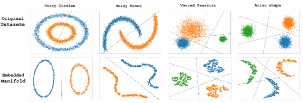
Although humans perceive the world in merely two-dimensional visual data, the brain is yet capable to comprehend the high-dimensional latent information beyond. The expression; “Where do we draw the line“ in the English language punted while debating a vague topic. The perception of two-dimensional data and the tendency to linearly separate the data are two technique leverage by humans in analytic. Likewise, the optical illustration of data visualization com- bined with dimension reduction techniques are the main reasons in the emerging of decision science based on big data in business, finance, and industry. Con- sider the upper row in Fig. 1; Four randomly-generated of 10000 data points in two-dimension. The attempt to fit linear regression lines through the data yields with at most 40% accuracy in classification of the color-annotated classes.
Stochastic Neighbor Embedding (SNE) [1] is a way to embed by high- dimensional data into a lower-dimensional space. SNE was culminated by its most successful version, the t-distribution Stochastic Neighbor Embedding (t- SNE) [2]. Despite both the computational and the memory complexity of t- SNE are bothO(n2), it demonstrated successful visualization of large real-world datasets with limited computational demands. The lower row of Fig. 1 illus- trated the datasets in the upper row after applying t-SNE for 50000 iterations
1Codes and more results can be found in: https://github.com/kkahloots/Improving-t-SNE- Visualization-and-Clustering
Figure 1: Four randomly-generated 2d datasets. The upper row shows the original datasets in 2d space. The lower row shows the embedded manifold after apply t-SNE. A linear separation attempt is carried out by linear regression.
of optimization by gradient descent. The embedded manifold is clearly linearly separated by the linear regression lines. Those forms of data in the embedded manifold are the simplest and can be learned by any linear classifiers with high accuracy.
For those relatively small datasets, it could not get any better results in fewer iterations. This raises some questions, which also were mentioned in the original t-SNE paper [2]. The first question is utilizing t-SNE in other purposes.
The t-SNE is a powerful visualization tool, however, it is not obvious how t- SNE will perform on the more general task of dimension reduction. Unlike Principal Component Analysis (PCA), the low-dimensional transformed data are not extrapolated to higher-dimensional data nor be modeled to transform another dataset. The second question is the curse of intrinsic dimensionality [3].
The t-SNE employs Euclidean distances between near neighbors, which operates under the premise that the underlying manifold has a local linearity property.
This appears clearly when applying t-SNE to CIFAR10 and CIFAR100 datasets, which encompass complicated objects in the images. The third question and the most troubling one is the non-convex property of the t-SNE cost function.
The objective of the t-SNE loss function is to minimize the Kullback-Leibler (KL) divergence between the embedded neighbor distribution and the high- dimensional neighbor distribution. In other words, it attempts to preserve the distances in relative low-dimensional embedding manifold with the respective original high-dimensional space.
The complexity arises in transforming the pairwise embedded distances into probabilities by projecting those distances on student t-distribution. The small change in the optimization parameter; e.g.-learning ratio, will lead to the total different embedded manifold. Therefore, a loss function with a lot of potential local minima can fail to capture the aspects of the original space and thatâs a weakness in t-SNE.
This paper organizes in six sections. The following section is the related work, in which previous methods to address t-SNE weakness are browsed. Sec-
tion 3 is a statistical preface of the mathematical equations in t-SNE model and a list of clustering metrics that has been used. Section 4 is the experimental setup and datasets description. section 5 is the results and discussion. Section 6 is the conclusion that shows the most effective values of the parameters to get best clustering and visualization.
2 Related Work
The upscaling of t-SNE was and still is the major weakness. Despite a quite long time, t-SNE has been published and available, it was an issue to scale up to large datasets with a reasonable amount of time until the fast interpolation- based t-SNE (Fit-SNE) have been emerged by G. Linderman et al. in [4]. In addition to C++ and memory optimized implementation, Fit-SNE is a fast Fourier transform (FFT)-accelerated interpolation-based t-SNE. This method rapidly computes of one-dimensional (1D) and 2D t-SNE based on polynomial interpolation and further accelerated using the FFT. The lead author of t-SNE, Laurens van der Maaten [5], came back with the best t-SNE implementation by using BallTree to measure distances, however, the Fit-SNE is using Approximate Nearest Neighbors (Annoy) method [6] which search for points in space that are close to a given query point. It also creates large read-only file-based data structures that are mapped into memory so that many processes share the same data.
The divergence for the t-SNE has been explored. D. Im et al. [7] attempted to ameliorate the issues non-convex objective function in the t-SNE criterion by studying the variational dual form such as KL, Reverse-KL (RKL), Jensen- Shannon (JS), Hellinger distance (HL), and Chi-square (X2). Basically, their work was an extension of work by Amid et al. [8] is closely related where they study Îą-divergences from an information retrieval perspective. Both studies concluded that optimization of the loss function is a trade-off visualization and parametrized that trade-off byα-divergences.
D. Kobak et al. [9] had replaced the Gaussian kernel by the heavy-tailed Cauchy kernel in an attempt to solve the âcrowding problemâ of SNE. It is a problem in the optimization by the gradient of the equidistant points. The combined gradients are so high so that those points will be squashed together.
The only drawback of this paper [9] is that it applied only to toy dataset, which does not suffer from the curse of intrinsic dimensionality (see the introduction).
G. Linderman S. Steinerberger [10] had proposed a new parameter for t-SNE that made it able to recover well-separated clusters. By automatically adjusting the early exaggeration precisely. Unfortunately, this parameter holds out only when the dataset is less than 20000 points. Moreover, this solution is equivalent to adaptive momentum of the gradient descent optimizer.
In this paper, we conducted a practical approach. The t-distribution per se can be tuned out to output a better visualization. In addition, the spatial nature of the embed manifold made it suitable for density-based spatial clustering. The purpose of the clustering we proposed is to find the purest and dichotomized
form of the manifold that also best representation. The target datasets are nearly real-world datasets of images.
3 Statistical Preface
In this section, the statistical concept are prefaced in addition to the clustering metrics that have been measured throughout later sections.
3.1 t-SNE Affinities
The affinities in the low dimensional space:
qij = wij
Z (1)
wij =k(kyi−yjk) (2) whereyis are the low-dimensional representation.
Then The Embedded ManifoldZ is:
Z =X
k6=l
wkl (3)
3.2 Gaussian Kernel
k(d) = 1
(1 +d2/α)α (4)
Whereαis the number of degrees of freedom of the student‘s t-distribution.
3.3 t-SNE Objective
t-SNE objective function is to minimize the KL loss as:
L=X
i,j
pijlogpij
qij (5)
Wherepij is symmetric and normalized affinity of pointxj and point xi
pij= pi|j+pj|i
2n (6)
andpi|j is the directional affinity over all points forj 6=i given as:
pj|i=
exp
− kxi−xjk2/2σi2 P
k6=iexp
− kxi−xkk2/2σi2 (7) The gradient of the loss function is:
∂L
∂yi = 4X
j
(pij−qij)wαij(yi−yj) (8) For a heavy-tailed t-distribution for t-SNE, αshould be asαâ (0, 0.5]
3.4 Clustering Metrics
Homogeneity, Completeness and v-measure are selected to evaluate the cluster- ing. In addition to Purity and Accuracy. Let C be a set of original classes in the dataset as:
C={ci|1, . . . , n} (9) K be a set of clusters
K={ki|1, . . . , m} (10) A br the contingency table produced by the clustering algorithm representing the clustering solution
A={aij} (11)
whereaijis the number of data points that are members of classciand elements of clusterkj .
Homogeneity is defined as:
h=
( 1 ifH(C, K) = 0
1−H(C|K)H(C) else (12)
where
H(C|K) =−
|K|
X
k=1
|C|
X
c=1
ack
N log ack
P|C|
c=1ack (13)
H(C) =−
|C|
X
c=1
P|K|
k=1ack
n log P|K|
k=1ack
n (14)
Completeness is symmetrical to homogeneity and defined as:
c=
( 1 ifH(K, C) = 0
1−H(K|C)H(K) else (15)
H(K|C) =−
|C|
X
c=1
|K|
X
k=1
ack
N log ack
P|K|
k=1ack
(16)
H(K) =−
|K|
X
k=1
P|C|
c=1ack
n log P|C|
c=1ack
n (17)
The V-measure is the harmonic mean between homogeneity and completeness:
Vβ =(1 +β)∗h∗c
(β∗h) +c (18)
whereβ is a scalar and usually β= 1
Clustering Purity is defined for a dataset withN data points, for a particular cluster is defined as: krof size nr
Figure 2: The upper row shows original two-dimensional space of the datasets;
MNIST, fashion MNIST, SmallNORB, CIFAR10, and CIFAR100. The lower row shows the embedded manifold by applying t-SNE withα= 1.
P(Kr) = 1 nrmax
i nir
(19) The overall purity of the clustering solution is obtained as a weighted sum of the individual clustering purity and is given by:
P urity=
k
X
r=1
nr
NP(Kr) (20)
The Clustering Accuracy is defined as:
accuracy(y,y) = maxˆ Pn
i=11{li=map(ki)}
n (21)
Where li is the ground-truth label, ki is the cluster assignment produced by the algorithm and map ranges over all possible one-to-one mappings between clusters and labels.
4 Experimental Setup
The target datasets are well-known image datasets and used widely in the re- search papers. The simplest is MNIST dataset, which is hand-written digits with 10 labels classes. The most complex is the CIFAR 100, which is a set of miscellaneous 100 labeled classes. All datasets have 60000 data points. The Fit-SNE was applied with regular t-distribution, i.e.-α= 1as mention equation 4. As shown in the lower row of Fig. 2, the t-SNE works quite fine with both MNIST and fashion MNIST but not that good for the rest of the datasets. Fur- thermore, there are no a small amount of unassigned data points inter-clusters, which make linearly separation is extremely incorrect. In the SmallNORB im- age, for instance, the yellow cluster (labeled as “human“) to the right-side is very adjacent to the red and the blue clusters. In addition, the yellow cluster is drifted apart to the right-side and to the left side of the manifold.
Figure 3: Clustering attempts for the datasets by using k-means, Spectral Clus- tering, GMM, and HDBSCAN. The lines are linear regression to separate one- vs-all classes.
After deliberation and experimentation, the alpha was set to 0.4. This selec- tion makes t-SNE a heavy-tailed kernel transformer that maximizes equation 5.
The visualization results were promising as shown in Fig. 3. The lingering task is to cluster the manifold space and measure the clustering metrics in equations 15,17,19 and 20. Seven clustering algorithms were applied on the embedded manifold; K-means [11], Spectral Clustering [12], Ward hierarchical Clustering [13], Birch Clustering [14], Gaussian Mixture Model [15], DBSCAN [16], and HDBSCAN [17].
5 Results and Discussion
Three objectives are sought by this paper; to generate an ecstatic visualization for the manifold and to cluster the manifold into homogeneous clusters and to be able to separate the clusters in a linear way. The objective of clustering the embedded manifold is to group the similar data points together. It is a possibility that the same labeled class be split into multiple clusters. The plau- sible explanation is that said labeled class has multiple pattern of data. The purity of a given resulting cluster indicate that this cluster has the same labeled class. Fig. 3 and Table 1 show clustering metrics for several clustering algo-
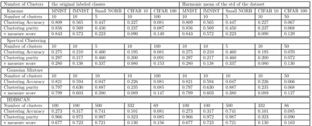
Table 1: Clustering metrics for the target datasets for original labled classes and for harmonic mean of the standard deviation of the data
Number of Clusters the original labeled classes Harmonic mean of the std of the dataset
Kmeans MNIST fMNIST Small NORB CIFAR 10 CIFAR 100 MNIST fMNIST Small NORB CIFAR 10 CIFAR 100
Number of clusters 10 10 5 10 100 10 10 5 10 50
Clustering Accuracy 0.809 0.565 0.447 0.227 0.081 0.809 0.565 0.447 0.227 0.067
Clustering purity 0.856 0.569 0.450 0.237 0.087 0.856 0.569 0.450 0.237 0.068
v measure score 0.843 0.572 0.223 0.090 0.149 0.843 0.572 0.223 0.090 0.129
Spectral Clustering
Number of clusters 10 10 5 10 100 10 10 5 10 50
Clustering Accuracy 0.275 0.210 0.460 0.195 0.081 0.275 0.210 0.460 0.195 0.070
Clustering purity 0.297 0.217 0.460 0.200 0.091 0.297 0.217 0.460 0.200 0.072
v measure score 0.280 0.138 0.337 0.080 0.153 0.280 0.138 0.337 0.080 0.130
Gaussian Mixture
Number of clusters 10 10 10 10 100 10 10 10 10 50
Clustering Accuracy 0.821 0.594 0.047 0.226 0.081 0.821 0.594 0.047 0.226 0.066
Clustering purity 0.797 0.630 0.887 0.235 0.085 0.797 0.630 0.887 0.235 0.068
v measure score 0.799 0.603 0.380 0.089 0.147 0.799 0.603 0.380 0.089 0.127
HDBSCAN
Number of clusters 100 100 500 332 69 100 100 500 332 86
Clustering Accuracy 0.273 0.317 0.741 0.101 0.081 0.273 0.317 0.741 0.101 0.085
Clustering purity 0.966 0.972 0.987 0.323 0.085 0.966 0.972 0.987 0.323 0.090
v measure score 0.677 0.723 0.721 0.130 0.156 0.677 0.723 0.721 0.130 0.163
rithms. Deciding the number of clusters is crucial clustering algorithms. When the number of clusters was set to be equal to the original labeled classes, all clustering algorithms gave out bad results. By understanding the nature of the manifold, the clustering task should not be subjective to the original labeled classes. Instead, the spatial condensed points should lay in the same cluster.
By relying on heavy-tailed t-SNE, the similar points are guaranteed to have small affinities in the manifold space.
Despite the good measurements of k-means and GMM clustering, as shown in 1, they failed in the visual objective because they have to cluster each and every point. On the other hand, the HDBSCAN clusters only spatially con- nected points and leave the perplexing points unclustered. By dropping the unclustered points from the manifold, the ecstatic visualization is achieved re- gardless of the losing about 5% of the data. Because the datasets are large scale, traditional t-SNE failed in allocating the required memory and carrying out the computations. On the other hand, the Fit-SNE uses the FFT transformation to interpolate. The 5% sparse data points inter-clusters are the downside of the Fit-SNE.
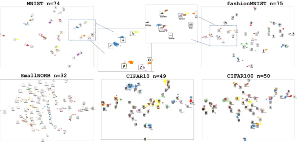
Fig. 4 shows the final results of clustering of the embedded manifold. HDB- SCAN successfully detected multiple clusters. The results by HDBSCAN make the ultimate sense and meets the clustering objective. For instance, the zero digits in the MNIST dataset have three patterns in this handwriting. Simi- larly, the six digits have three patterns too. Fig. 4, in the middle of the upper row, shows multiple detected patterns for the same labeled classes. The class âsandalâ has four patterns in the fashion MNIST dataset and they have been detected successfully.
Figure 4: Clustering for the datasets by using HDBSCAN. The number of clus- ters was set by the harmonic mean of the standard deviations of the images, Nonetheless, HDBSCAN has detected the clusters based on spatial densities. In the upper row, zoom in for sub-manifold that is demonstrating multiple patterns for the same class label.
6 Conclusion
In this paper, t-SNE had been demonstrated to be unsuited for large datasets, whilst the Fit-SNE was efficient only be adjusting the degree of freedom to be 0.4. The clustering of embedded manifold for the famous datasets MINIST, fashion MNIST, SmallNORB, CIFAR10, and CIFAR100 has been investigated thoroughly. The most successful clustering was HDBSCAN due to its spatial mechanism to glue points together and due to its ability of drop out the spars inter-clusters points. The resulting clusters had detected several patterns for the same labeled classes. In addition, the visualization was ecstatic and the clusters were well-distinguished.
Acknowledgment
This work was performed in the frame of FIEK 16-1-2016-0007 project, implemented with the support provided from the National Research, Development and Innovation Fund of Hungary, financed under the FIEK 16 funding scheme. It was also supported by the BME Artificial Intelligence FIKP grant of EMMI (BME FIKP-MI/SC) and by the Janos Bolyai Research Fellowship of the Hungarian Academy of Sciences.
References
[1] Geoffrey Hinton and Sam Roweis. Stochastic neighbor embedding. InProceedings of the 15th International Conference on Neural Information Processing Systems,
NIPS’02, pages 857–864, Cambridge, MA, USA, 2002. MIT Press.
[2] Laurens van der Maaten and Geoffrey E. Hinton. Visualizing data using t-sne.
2008.
[3] Yoshua Bengio. Learning deep architectures for ai. Foundations and TrendsÂŽ in Machine Learning, 2(1):1–127, 2009.
[4] Jeremy G. Hoskins Stefan Steinerberger George C. Linderman, Manas Rachh and Yuval Kluger. Fast interpolation-based t-sne for improved visualization of single-cell rna-seq data. Nature Methods, 16(3):243–245, 2019.
[5] Laurens van der Maaten. Accelerating t-sne using tree-based algorithms.Journal of Machine Learning Research, 15:3221–3245, 2014.
[6] Alexandr Andoni, Piotr Indyk, and Ilya P. Razenshteyn. Approximate nearest neighbor search in high dimensions. CoRR, abs/1806.09823, 2018.
[7] Daniel Jiwoong Im, Nakul Verma, and Kristin Branson. Stochastic neighbor embedding under f-divergences. CoRR, abs/1811.01247, 2018.
[8] Ehsan Amid, Onur Dikmen, and Erkki Oja. Optimizing the information retrieval trade-off in data visualization using $α$-divergence.CoRR, abs/1505.05821, 2015.
[9] Dmitry Kobak, George C. Linderman, Stefan Steinerberger, Yuval Kluger, and Philipp Berens. Heavy-tailed kernels reveal a finer cluster structure in t-sne visu- alizations. CoRR, abs/1902.05804, 2019.
[10] George C. Linderman and Stefan Steinerberger. Clustering with t-sne, provably.
CoRR, abs/1706.02582, 2017.
[11] D. Sculley. Web-scale k-means clustering. InProceedings of the 19th International Conference on World Wide Web, WWW ’10, pages 1177–1178, New York, NY, USA, 2010. ACM.
[12] Yu and Shi. Multiclass spectral clustering. InProceedings Ninth IEEE Interna- tional Conference on Computer Vision, pages 313–319 vol.1, Oct 2003.
[13] Fionn Murtagh and Pierre Legendre. Ward’s Hierarchical Clustering Method:
Clustering Criterion and Agglomerative Algorithm. arXiv e-prints, page arXiv:1111.6285, Nov 2011.
[14] Tian Zhang, Raghu Ramakrishnan, and Miron Livny. Birch: An efficient data clustering method for very large databases. SIGMOD Rec., 25(2):103–114, June 1996.
[15] Christopher M. Bishop. Pattern Recognition and Machine Learning (Information Science and Statistics). Springer-Verlag, Berlin, Heidelberg, 2006.
[16] Martin Ester, Hans-Peter Kriegel, JĂśrg Sander, and Xiaowei Xu. A density- based algorithm for discovering clusters in large spatial databases with noise.
pages 226–231. AAAI Press, 1996.
[17] Leland McInnes and John Healy. Accelerated hierarchical density clustering.
pages 33–42, 05 2017.