Visual feature recognition based indoor localization ∗
Sándor Plósz
a, Csaba Lukovszki
b, Gergely Hollósi
aaBudapest University of Technology and Economics plosz@tmit.bme.hu
hollosi@tmit.bme.hu
bInter-University Centre for Telecommunications and Informatics lukovszki@etik.hu
Abstract
Existing indoor localization solutions require an expensive, pre-installed infrastructure. On the other hand the advancements in the area of computer vision, in particular in feature recognition, extraction and matching algo- rithms makes this approach interesting to be investigated. Modern feature detection algorithms are able to extract features which are strong, unique and invariant to rotation and scaling, so the array of these features represent an image well. By finding similarity between images based on comparing features we are able to detect if images have been made from different viewpoints of a single scene. In this work we have set up a test environment to investigate some of the most popular feature detection algorithms and methods on a real indoor dataset for their usability for visual localization.
Keywords:Visual recognition, computer vision, localization, feature detection MSC:AMS classification numbers
1. Introduction
The demand for indoor localization in the commercial environment have been in- creasing in the past years as outdoor localization became mature and part of peo- ple’s everyday life. The appearance of smart phones has opened a new platform for leading technological evolution. Markers are placed inside commercial buildings
∗Held on the hosted workshop: “Workshop on Smart Applications for Smart Cities”.
Bay Zoltán Nonprofit Ltd. for Applied Research Eger, Hungary, November 5–7, 2014. pp. 143–150
doi: 10.17048/FutureRFID.1.2014.143
143
Figure 1: Feature detection methods
which can be read by the camera for displaying related information, can also be used for telling the location of the user.
Our approach is to use a photo created by the smart phone’s camera to find the location of the user. By extracting visual features it is possible to make comparisons of images to find similarities. If we have mapped the environment for images and created a dataset where we have also stored the location where the images were made we can compare an image against this dataset to find the most similar ones.
Based on this we can estimate the position the image was made.
In our previous work [8] we have evaluated the performance of the feature detection algorithms using brute-force pairing. In this work we examine a more effective method for comparing images.
Visual features has been previously used for many applications, including clas- sification for object detection [2], robot navigation [9], augmented reality [5] and image search using a visual vocabulary [11].
At first in section 2 we describe how feature based matching actually works, what are the main steps and how we have performed it. In section 3 we describe the evaluation environment we have set up to test the described methods. The results of the evaluation are given in section 4. After that, in section 5. we discuss how this works fits into the big picture of creating a visual localization system.
Finally, in section 6. we conclude the paper.
2. Visual Feature based matching
Our goal for achieving localization was to find a way to be able to compare images.
Visual features can represent an image, therefore it can also be used to compare images. There are three types of visual features: points, edge, and blob. Also there are different kind of algorithms which can detect features on images, in the form of intensity changes (gradients).
The process of working with visual features to be able to do comparison is depicted in figure 1. First an algorithms detects visual features on an input image.
Then these features are each described in a vector format. Since an image can have hundreds of detected features, for a large dataset it is not always feasible to store all the features, so different feature storing methods have been developed. One of them is the Bag of Features (BoF), which is detailed below.
Two images are compared by matching (pairing) their features one-by-one. For a feature its pair will be its nearest neighbour, which is within a threshold distance.
The distance measure depends on the algorithm, but most commonly Euclidean (L2) distance is used. The more features can be paired the more similar the two images are likely to be. Not all features can be paired right, however. The fact that the image pairing method is a homography (projective mapping) can be used to rule out incorrect matches, which are also called outliers. This only works if the number of correct matches are considerably larger than the incorrect ones.
2.1. Visual feature detection
Visual feature detection algorithms work by detecting intensity changes on gray- scale images. Beside the location of the feature on an image, modern algorithms also detect scale, and orientation.
In this work we have worked with four different feature detection algorithms:
• Harris detector [3] is based on the autocorrelation of the image to detect significant intensity changes. Calculating autocorrelation is a processing de- mand tasks which is approximated with the so called Harris operator con- sisting the two way gradients of the image. For every pixel of the image the Harris matrix has to be made, its determinant and trace will determine whether it is a feature point or not. The operation of the Harris detector is highly influenced by the scale and rotation of the image.
• Scale-invariant feature transform (SIFT) is a feature detection method based on the difference of Gaussians and Laplacian of Gaussian filters [6]. In fact, the image is convolved with Gaussians of different variance, and subtracted from each other. This operation is performed on different scales to achieve scale invariance. The SURF (Speeded Up Robust Features) algorithm is similar to SIFT except it uses a so called Fast-Hessian detector [1].
• The Maximally stable extremal regions (MSER) method is a popular blob detection technique [7]. Regions in an image consists of pixels having intensity below a certain threshold. As this threshold is increased more and more regions start to form, extend and merge. The algorithm keeps track of these regions, they number, the rate they grow and how they merge. Some regions tend to be stable meaning the rate they grow is minimal. Based on these numbers the algorithm selects the most stable ones against the change of threshold. MSER reacts well to image scaling and rotation so it is widely used nowadays.
• Features from accelerated segment test (FAST) method involves training a decision tree with attribute vector of 16 pixel intensity values, which are in
Clustering Marker feature
matrix Marker images
64 dimension vectors Marker image feature
vectors
1 2 3 4 5
Histogram
5 4 3 2 1
2 5 4 2 1 4 2 2 5 Cluster indexes
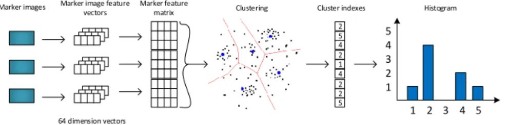
Figure 2: BoW clustering method
a circle of radiusr around the candidate point [10]. Corners are identified based on how the surrounding pixels compare with the center pixel. The study point is a corner if there are 12 consecutive pixels from the perimeter that are consistently brighter or darker than the center by a threshold T. To make the algorithm fast, first the intensity of pixels 1, 5, 9 and 13 of the circle are compared to the center. If at least three of the four pixel values (I1,I5, I9, I13) are not in the (Ip+T, Ip−T) interval, then the algorithm checks for all 16 pixels and examines the 12 contiguous pixels failed in the criterion above.
2.2. Bag of Words method
The Bag of Words (BoW) is a method for clustering the numerous features repre- senting an image. This way an image is represented by one vector instead of many.
This not only reduces the storage requirement of the features but also the time the feature matching takes, thereby increasing scalability.
In BoW method the vector space of features is divided to pre-defined number of clusters, which are identified by their centers. The division takes place by clustering an initial vector set, which are the features of images stored in the database for comparison. The most popular algorithm which achieves this is the K-NN (K neirest neighbors). The algorithm works as follows:
1. Select N number of vectors which will be the initial cluster centers. In our case,N is the number of clusters.
2. Determine for each other vector their nearest cluster center.
3. Select new cluster centers which are nearest to the geometric center of the vectors in each cluster.
4. Jump to step 3. until the centers remain unchanged.
The K-NN algorithm clusters each feature vector to one of the clusters. This is followed by calculating a histogram from the number of feature vectors assigned to each cluster. This histogram will be the new vector representation of the image.
The method is depicted in figure 2.
Since the numbers of the histogram vector depends on the number of features an image has it has to be normalized to become comparable. This is because there can two images made from slightly different viewpoints, where one of the viewpoints contains an object with a lot of edges, which will result in a large number of features.
When normalized, these fill just represent one value in the histogram rather than a large number.
Histograms are usually compared based on their Euclidean distances.
3. Evaulation of methods
We have set up a test environment to evaluate visual feature recognition based methods for localization. First we have created a test dataset containing images taken at 25 different locations. This dataset can be divided into two groups: mark- ers and samples. Markers are taken at the mapping stage of the environment.
They are high resolution, good quality images taken under ideal light conditions, close-up, upfront the scene and one or two angles. Samples represent query images taken under less ideal conditions, farther of the scene and from random angles. In this dataset a localization method has to find the location of a query image by finding the marker image taken at the same place.
First we process the marker images by performing clustering with different cluster sizes, then determine the cluster centres and calculate their histogram vector representation. Then also for each sample image we perform clustering, calculate the histogram vector and compare it to all the marker histogram vectors for finding the one with the minimal Euclidean distance. If that marker has been made at the same location as the sample image, we call it a positive match. We create statistics for the ratio of positive matches for evaluating a scenario, which comprises different algorithms and cluster sizes.
We have used the Matlab environment for performing the evaluation. Recent Matlab releases contain the computer vision toolbox, which have several feature detection algorithms embedded. We have written a script in Matlab for reading the dataset, detecting features, performing clustering, matching histograms, and calculating statistics of positive matches as well as processing times.
4. Results
In the literature we have encountered quite large cluster sizes, the minimum limit is of course the number of images, otherwise there will be two vectors which are the same, therefore the number of clusters should be much higher than the number of markers. We have selected the following cluster sizes to evaluate: 500, 1000, 2500,
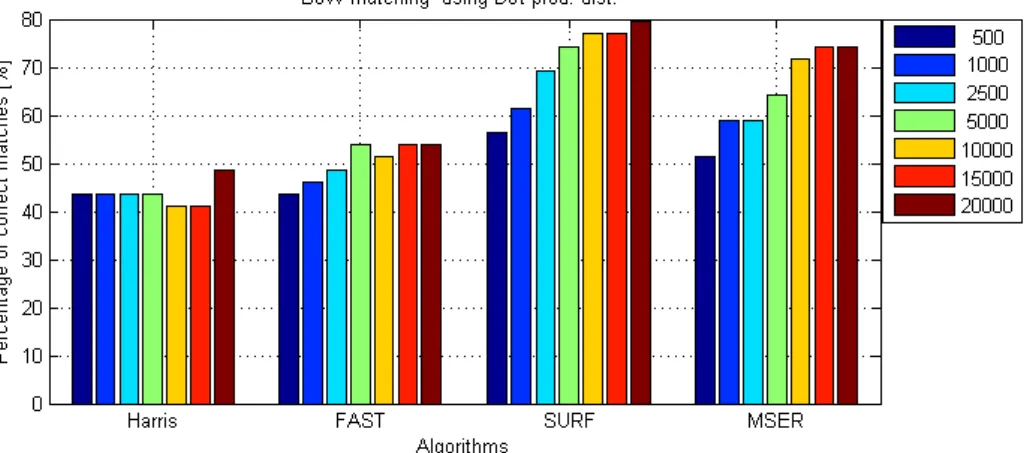
Figure 3: Positive match statistics with BoW clustering method
5000, 10000 and 15000. Since the time and memory requirement increases linearly with the size of the cluster and the number of feature vectors, using larger clusters are only computable if we reduce the number of feature vectors to be clustered.
For example, in Matlab, clustering with 10000 sized clusters needs almost 5GB memory. With larger cluster sizes we have to reduce the number of vectors with random selection. For example, the combined marker feature list contained about 110.000 elements. For clustering with 15000 clusters we had to reduce this set to half, e.g. we selected about every second element. Filtering in this level should not reduce the accuracy of the evaluation.
The results of the evaluation are depicted in figure 3. As in our previous in- vestigation where we used brute-force matching technique to compare images, the SURF algorithm proved to be the best, achieving 79% positive match for 20000 clusters. We could not increase the cluster size any further due to the excessive memory requirement.
Beside the achievable precision we have also examined the time requirements for performing the matchings. From a sample image until finding the closest marker the following operations have to be performed:
• Detect features of the image
• Cluster the features and calculate the BoW representation
• Compare the BoW vector to all the vectors of marker images and get the closest one
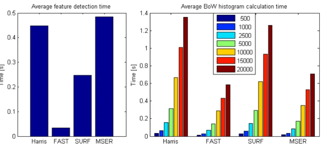
Among these the first two has noticeable time requirements while the time for search among vectors can be considered negligible, after all this was the point of using the BoW approach. The processing times averaged for all the sample images are shown in figure 4. We can see that the histogram calculation time increases
Figure 4: Average feature detection and BoW calculation time for different cluster sizes
exponentially with the cluster size and can easily exceed the feature detection time.
Also, though MSER has higher detection time than SURF, clustering is faster for MSER features. For comparison, with SURF and 15000 clusters we can achieve 77%
precision with 1.2s processing time, for a 2% increase, using 20000 clusters it needs 1.5s. In these comparisons we haven’t mentioned the cluster center calculation time, because it has to be performed once, but it is the longest process, takes about 110s for 15000 clusters, and 140s for 20000 clusters.
5. From visual features to localization
When pairing images, the relation of the features is also an important information.
The geometric relation of the features is a homography which can be used to estimate the spatial relation of the cameras that have taken the images (up to a scale) [4]. From this the problem is geometric. In order this to work we have to work on reducing the number of false positive matches given by the currently used metric of maximum score selection. We will be focusing on this in the future.
6. Conclusions
In this work we have evaluated similar image search using different feature detection algorithms and Bag of Words description method working with clustering feature descriptors. The provided single histogram vector proved to be a usable repre- sentation of an image for finding similarities. We have run tests using different, increasing cluster sizes, and experienced improvement in the precision of finding a correct match based on our simple metric. By examining the processing memory
and time demand we experienced an exponential increase with increasing cluster sizes. There is a trade-off between these values which depends on the processing unit and the size of the dataset.
To conclude the BoW approach is a usable method for feature description which increases scalability a great deal, resulting about 20% loss in precision of finding correct matches.
References
[1] Herbert Bay et al. “Speeded-Up Robust Features (SURF)”. In:Comput. Vis.
Image Underst.110.3 (June 2008), pp. 346–359.
[2] O. Chum et al. “Total Recall: Automatic Query Expansion with a Generative Feature Model for Object Retrieval”. In:Computer Vision, 2007. ICCV 2007.
IEEE 11th International Conference on. Oct. 2007, pp. 1–8.
[3] C. Harris and M. Stephens. “A Combined Corner and Edge Detector”. In:
Proceedings of the 4th Alvey Vision Conference. 1988, pp. 147–151.
[4] R. I. Hartley and A. Zisserman.Multiple View Geometry in Computer Vision.
Second. Cambridge University Press, ISBN: 0521540518, 2004.
[5] Taehee Lee and T. Hollerer. “Hybrid Feature Tracking and User Interaction for Markerless Augmented Reality”. In:Virtual Reality Conference, 2008. VR
’08. IEEE. Mar. 2008, pp. 145–152.
[6] D.G. Lowe. “Object recognition from local scale-invariant features”. In:Com- puter Vision, 1999. The Proceedings of the Seventh IEEE International Con- ference on. Vol. 2. 1999, 1150–1157 vol.2.
[7] J Matas et al. “Robust wide-baseline stereo from maximally stable extremal regions”. In:Image and Vision Computing 22.10 (2004), pp. 761–767.
[8] S. Plosz et al. “Practical aspects of visual recognition for indoor mobile po- sitioning”. In: Cognitive Infocommunications (CogInfoCom), 2013 IEEE 4th International Conference on. Dec. 2013, pp. 527–532.
[9] Arnau Ramisa et al. “Robust vision-based robot localization using combina- tions of local feature region detectors”. In: Autonomous Robots 27.4 (2009), pp. 373–385.
[10] Edward Rosten and Tom Drummond. “Machine Learning for High-Speed Corner Detection”. In: Computer Vision – ECCV 2006. Vol. 3951. Lecture Notes in Computer Science. Springer Berlin Heidelberg, 2006, pp. 430–443.
[11] Shiliang Zhang et al. “Building Contextual Visual Vocabulary for Large-scale Image Applications”. In:Proceedings of the International Conference on Mul- timedia. MM ’10. 2010, pp. 501–510.