Extrapolation of Saturated Diffraction Spikes in Photographs Containing Light Sources

(1)

Cite this article as: Pizág, B., Nagy, B. V. "Extrapolation of Saturated Diffraction Spikes in Photographs Containing Light Sources", Periodica Polytechnica Mechanical Engineering, 64(3), pp. 233–239, 2020. https://doi.org/10.3311/PPme.16044

Extrapolation of Saturated Diffraction Spikes in Photographs Containing Light Sources

Bertalan Pizág^1*, Balázs Vince Nagy¹

1 Department of Mechatronics, Optics and Mechanical Engineering Informatics, Faculty of Mechanical Engineering, Budapest University of Technology and Economics, H-1521 Budapest, P. O. B. 91, Hungary

* Corresponding author, e-mail: pizag@mogi.bme.hu

Received: 20 March 2020, Accepted: 18 May 2020, Published online: 29 June 2020

Abstract

The observed luminance of most light sources is many orders of magnitude higher than the luminance of surrounding objects and the background. With the dynamic range of single photographs limited to 8 to 10 bits, both dark and bright values are radically coerced to the limits. This problem is usually circumvented with the use of High-Dynamic-Range (HDR) imaging, assembling multiple photographs of the same scene made at different exposures. But in some situations, or due to equipment limitations, HDR imaging might not be possible. This research is aimed at the extrapolation of luminance peaks within oversaturated Low-Dynamic-Range (LDR) images. The proposed method of extrapolation relies on the identification and analysis of Fraunhofer diffraction patterns created by the aperture. The algorithm is tested on a set of HDR images containing one or two lamps. These images are converted to LDR at a custom saturation cap, then extrapolated to restore the original peaks with relative success.

Keywords

image processing, photometry, Fraunhofer diffraction, luminance measurement

1 Introduction

Throughout this article, we propose a method for the estimation of luminance peaks on oversaturated photographs containing different light sources.

To achieve this, we rely on the Fraunhofer diffraction patterns [1–6], often called diffraction spikes [7], created by the aperture of the imaging system. The size of the patters depend mainly on two factors: the luminance of the observed source and the geometrical features (shape and size) of the apertures [2]. These patterns are generally considered aberrations in imaging systems, and considerable effort is made to correct them, usually by measuring/calcu- lating the Point Spread Function (PSF) and using deconvolution methods to deblur the image [8, 9]. In extreme cases, such when bright sources are present in the image, these patterns become too large for usual deconvolution but can be analyzed with other image processing methods. In this article, we identify parts of these patterns and extrapolate them into the saturated regions to reconstruct the missing peaks.

The article presents the developed method in two separate steps. At first, the diffraction spikes are identified by extracting the saturated parts of the image and filtering for valid shapes then the surrounding gradients are

propagated into the region, forming a skeletal structure of the spike. A primitive pattern of the spike is fitted onto the skeleton to determine its orientation. Then sections of the image are taken at the arms of the distribution and in-between. In the second step, these sections are analyzed using the mathematical theory of diffraction, and curves are fitted onto them to reconstruct the missing region.

In the end, we compare the extrapolation results to the original values.

2 Methodology

In Section 2, we present the developed method in two separate parts, the first dealing with the image processing and feature extraction, and the second dealing with the models used for the curve fitting and peak estimation. The calculations were performed using MATLAB [10].

2.1 Extraction of diffraction spikes

The aim of the extraction process is to locate each diffraction spike on the image, determine their center points, their orientation, and create slices along the identified arms and in-between them.

(2)

While it is not necessary to determine the orientation on an individual basis, as it is a constant value, influ- enced only by the aperture [1], we decided to calculate it for each source to increase robustness and possibly correct for small mistakes in the center point identification.

The current version of the model can handle multiple sources present in the same image; however, their saturated regions should not overlap, and each one should be located well within the image boundaries.

The parameters for the various functions were experimentally determined for the camera setting used in the experiments. As far as the experiments have gone, it is safe to say that a single parameter setup is sufficient for a camera configuration (fixed focus and aperture with exposure time depending on pattern size).

2.1.1 Image filtering and gradient vectors

At the very first step, the image is zero-padded to pre- vent runtime exceptions caused by near-border operations (should not affect proper shots), then a Gauss-blur is applied to reduce noise. After this step, both directional gradients are calculated using 3 × 3 Sobel operators [11]. These gradients are then formed into unit vectors representing their direction; their magnitude is ignored in the calculations.

2.1.2 Source separation

Parallelly, a binary mask is created based on the original, unblurred image containing the saturated pixels.

We remove spots that are too small to be separate sources (usually lens flare), then count and separate the remaining ones into new masks. From this point on, the process is repeated for each identified source independently. After the separation, the images are cropped to their relevant domain, then the internal holes of every mask is filled in.

2.1.3 Gradient source generation

The aim is to propagate the gradient vectors into the saturated area, which lacks any proper image information.

To this end, a starting area is designated for the calculations by dilating the mask multiple times, then dropping the innermost layer. This way, the starting gradients are placed on the sides of the pattern, which are close enough not to be disturbed by other sources in the image, but far enough that the blurring won't feed false data (saturated pixel values) into them.

2.1.4 Gradient propagation

The propagation of the gradients into the saturated region is necessary, as the available parts of the arms provide

unreliable information about the orientation of the pattern. Using the gradients all around the pattern for feature extraction makes the algorithm more robust.

We have devised a simple method for propagating the gradients into the saturated region while preserv- ing the straight edges pointing inwards along the arms;

the process is summed up in Algorithm 1. We project the 3 × 3 neighborhood of the gradient vector to unit vectors pointing towards the selected pixel, as shown in Fig. 1 if there is at least three non-zero value among them, then the resulting vectors are summed and normalized to create the new unit vector at the pixel location, and it is flagged as a valid gradient. The program iterates over the image until all pixels receive gradient vectors, or the process is stuck (should not happen with proper images).

As a result, the borders between the regions are pre- served and pushed inside of the saturated area, as seen in Fig. 2. Although some false edges can appear as well along the main directions of the projection.

Algorithm 1 Gradient propagation

V[x, y] ← Calculate unit vectors for the whole grid;

M[x, y] ← Mask the designated area;

N ← 0;

while

∑

M^≠⁰^do N←

∑

M ^; M_old ← M;

V_old ← V;

foreach i in [xmin₊1,xmax₋1] do foreach i in [ymin₊1,ymax₋1] do

if Mold (i, j) = 0 then

n ← Sum 8 neighborhood around M_old (i, j);

if n ≥ 3 then M(i, j) ← 1;

m[3, 3] ← Project vectors in the 8 neighborhood at the unit vectors pointing towards V_old (i, j);

V i j( ), ←^norm

( ∑

m

)

^;

end end end end

if

∑

M N⁼ ^then break;

end end

(3)

2.1.5 Edge and center point search

The edges between the regions are found using a criterium for the number of inward-pointing projected vectors. If at least five of the eight vector components point towards the center, the pixel is considered to be an edge compo- nent. We have considered using the ratio of total incoming value compared to the total absolute value, but this method proved unreliable at detecting finer details.

We preferred this method to more conventional binary image skeletonization [11, 12], as false negatives were much rarer for the arms, while the pattern fitting handled the increased number of false positives. This is shown in Figs. 2. and 3.

Similarly, the center point was located by find- ing the pixels with the most inward-pointing gradients.

This search was limited to the proximity of the image center, as lens flare spots could be interpreted as center points too. The centroid of the eligible pixels was designated as the center of the diffraction spike.

The small unconnected edge parts were removed so they won't disturb the orientation fitting.

2.1.6 Oriented pattern fitting

The shape of the PSF, therefore the diffraction pattern is dependent on the shape of the aperture. For straight edge regular polygons, these shapes are pointy start with arms either the same (even) or double (odd) the number of the sides [3, 5, 13]. However, the model becomes significantly more complicated if the edges of the polygons, as in the case of usual camera apertures, are slightly curved [13–16]. Our cameras used in the experiments had slightly curved hexagonal apertures, but we used the straight edge model for calculations, as it is available as a closed-form equation [3, 6].

The orientation was determined by placing a Gauss- blurred three-line star shape over the center point, aver- aging the covered values at different angles. The best-fitting version was declared to be the pattern's orientation, as seen in Fig. 3.

2.2 Curve fitting

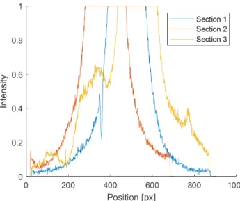
The second step of the processing method involves slic- ing the images along the identified lines and also along their angle bisectors, extracting pixel information along the lines, as seen in Fig. 4, then approximating the diffraction spots based on the sections.

2.2.1 Creating the sections

The slices are extracted starting from the center point to the image borders and converted to distance-based data.

Due to the symmetry of the patterns [5], these sections align well with the others in the same category.

Fig. 1 The vectors used for the projection (a) and the process of the gradient propagation (b)

Fig. 2 The extrapolated gradient angles (a) and the skeletonized edges with the center point (b)

Fig. 3 Estimated arm directions on the skeleton (a) and on the saturated shape (b)

Fig. 4 Sections of a diffraction spike along the arms, the small peaks in Section 3 are the results of lens flare

(4)

2.2.2 Curve fitting

The characteristics of the diffraction spikes can be approx- imated by fitting functions to these sections.

The shapes of the functions are chosen to represent the mathematical model of Fraunhofer diffraction patterns observed at hexagonal apertures [2, 3, 6]. According to [2]

and [6], the diffraction pattern of the aperture takes on the shape presented in Eq. (1).

ψ χ

χ π

x nx

ix n j

n j ,

exp cos

sin s

( )

=

−  −

 











−

(

−

)









2

2 1

2

iin

, χ π−

(

+

)









∑

=

n j

j n

2 1

1

(1) where x is the radial coordinate of the diffraction pattern, normalized by wavelength and weighed by the aperture radius, χ is the polar angle, and n is the number of sides of the polygon.

Equation (1) is further simplified, as explained in [2]

and [3], if the polygon is even-sided and if the polar angle matches either of our selected directions.

These equations, however, describe patterns that are not monotonously descending but contain a repeated series of peaks, because the models only consider a single wavelength. For each wavelength, the distance between the interference peaks changes, while their intensity remains approximately the same. The white-light diffraction patterns can be interpreted as the superposition of single wavelength models [4], and their enveloping function can be used to estimate the pattern characteristics.

We assume that the envelope function follows the characteristics of the decreasing local maxima values, which means 1/x characteristics for the arms, and 1/x² characteristics for the rest of the sections [6]. To allow for better fitting, we have extended these functions with additional constants, as presented in Eqs. (2) and (3).

Iarm =a x b₁

(

+ ₁

)

+c₁ (2) Ibisec =a2

(

x b+

)

⁺c

2

2 2 (3)

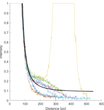
These functions are fit over the merged data of each section type using the nonlinear least-squares method, so the same function is applied to all six directions to address the symmetry. The fitting ignores the saturated region and everything further than three times the saturated radius, so it ignores further peaks present in the data, as present in Fig. 5.

2.2.3 Centerpoint estimation

The parameter of the resulting functions is negative in the overwhelming majority of the cases, making the function value rise to infinite before the origin. Most parts of the curve can be used to estimate the pattern, but the peak still can not be restored.

The function, therefore, is capped by inserting a simple, spike-shaped function tangential to the fitted curves.

We have tested Gauss, Dirac delta, and sinc functions, but their fitting proved difficult. Instead, we simply used a tri- angular function fit tangentially to the curves at a designated gradient angle.

Throughout our experiments, we came to the conclusion that this angle is dependent mostly on the camera configurations and gives relatively reliable results in measurements conducted under similar conditions.

3 Experimentation

We have tested the algorithm on a set of different halo- gen lights to set up the system parameters and estimate its reliability.

3.1 Testing dataset

For the testing, we have created a dataset of 200 images containing halogenic lamps equipped with two differently shaped reflectors or none at all. At a time, only one or two sources are present in an image.

Fig. 5 Sections along the bisectors and the fit results of the 1/x² function

(5)

The images were taken using a Basler ace acA800-510um monochromatic camera with a resolution of 832 × 632 pixels and 10-bit depth. Each scene was recorded with multiple exposures and assembled into HDR images [15, 17], where every single pixel contains valid information (not saturated or below noise level). The exposure times increase by a factor of 2 with each new take, and for each pixel, the highest non-saturated value is selected, then weighed back to the shortest exposure time.

The camera controller and HDR image assembler application was built in Python 3.7, using the Basler pypylon and NumPy [18] libraries.

3.2 Data preparation

The HDR images were converted back to LDR ones by capping their values at a certain level, simulating the saturation, and the remaining data were scaled up and resampled to 8 or 10-bit linear representation.

This way, the extrapolated peaks can be compared to the real results without requiring repeated measurements or different reference instruments.

Both the HDR and LDR images are represented with double precision floating point numbers between 0 and 1 to reduce sampling errors and minimize the need for type and range conversion.

3.3 Results

The detection and feature extraction of the diffraction spikes proved extremely robust, working properly for all tested lamp types as long as they were well within image boundaries (partial patterns failed at the orientation matching step) with visible arms.

The sections, therefore, contained the proper data sets for the curve fitting in essentially all of the valid testing images.

The fitted functions, in most cases, matched the LDR images but diverged slightly from the HDR ones inside the region of extrapolation: the 1/x function aligns well with the wider spots of the reflectors, often deviating when no such components exist, as presented by Fig. 6. In contrast, the 1/x² aligns more closely to the peak, but behaves less predictably. We consider these to be the effect of using point source models to estimate extended source characteristics.

The peak estimation at the end of the process is subject to significant errors from a metrological standpoint, as the peak estimate is located between 0.2–5 times the original value, occasionally deviating by more than an order

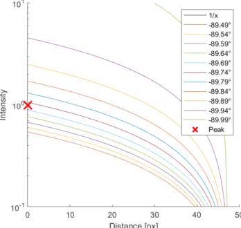
of magnitude. But this accuracy is still formidable if we consider how steep were the gradients used for the estimation, as seen in Fig. 7.

For obvious reasons (higher gradient) the 1/x² curves proved less effective at peak estimation, but the 1/x curves provided consistent results throughout the entire dataset.

Based on the experiments, these angles mainly depend on the camera configuration; their uncertainty is related to the precision of the feature extraction and curve fitting.

Fig. 6 Deviation of the 1/x function from the original data, this effect, surprisingly, does not influence the peak estimation

Fig. 7 Gradient lines intersecting the Y-axis around the original peak.

(6)

There was a multitude of error sources not considered throughout the modeling. The problem of extended sources was experimentally included in the fitting model, but not to the extent that diffuse sources could be modeled.

The current method is functional only for light sources with small regions of intense luminance.

Similarly, the camera response function [19–21] was assumed to be ideal and was not corrected; this can, however, cause serious deviations around the peaks [21].

Furthermore, the spectral composition of the spots was also ignored by assuming homogeneous luminance through the entirety of the visible spectrum.

4 Discussion

Throughout the article, we have proposed a method for the detection and analysis of saturated diffraction spikes with the purpose of reconstructing the missing data.

However, we built this upon experimentally tuned models.

These models require even more extensive testing, along with methods for their parametrization before the system can be given any practical use.

The results are promising and, by refining the mathematical models and eliminating disturbing effects from the original image, the accuracy might be significantly improved. However, the gradient problem would still remain, and any small uncertainty in the curve fitting would radically distort the result.

For future improvement, a more mathematics heavy approach could be taken by including the measurement and application point spread function and deconvolution based method. Possibly a harder to compute machine-learn- ing based approach could also handle extended sources,

though the steep gradients would definitely lead to an excess of false positives.

And for any serious metrological application, the camera response function has to be taken into account, along with image defocus effects and aberrations.

5 Conclusion

Throughout this article, we have proposed a two-stage method for the extrapolation of saturated image data based on Fraunhofer diffraction patterns. The first stage con- sists of a robust detection and feature extraction algorithm based on gradient propagation into the missing region, while the second stage aims to reconstruct the data by fitting various functions on the available data.

The results did not prove fit for metrological use, being often just within an order of magnitude away from the peak value, but most of the region could still be recon- structed with fairly great accuracy, and there is still significant potential for further improvement.

Acknowledgment

Balázs Vince Nagy was supported by the János Bolyai Scholarship of the Hungarian Academy of Sciences.

The research reported in this paper has been supported by the National Research, Development and Innovation Fund (TUDFO/51757/2019-ITM, Thematic Excellence Program).

The research reported in this paper was supported by the Higher Education Excellence Program of the Ministry of Human Capacities in the frame of Artificial Intelligence research area of Budapest University of Technology and Economics (BME FIKP-MI/FM).

References

[1] Marathay, A. S. "Physical Optics: Chapter 3 - Diffraction", In: Bass, M. (ed.) Handbook of Optics, Volume I, McGraw-Hill, New York, NY, USA, 1995, pp. 187–217.

[2] Komrska, J. "Fraunhofer Diffraction at Apertures in the Form of Regular Polygons. I.", Optica Acta: International Journal of Optics, 19(10), pp. 807–816, 1972.

https://doi.org/10.1080/713818504

[3] Komrska, J. "Fraunhofer Diffraction at Apertures in the Form of Regular Polygons. II", Optica Acta: International Journal of Optics, 20(7), pp. 549–563. 1973.

https://doi.org/10.1080/713818798

[4] Bergsten, R., Popelka, S. H. "White-light Fraunhofer diffraction", Journal of the Optical Society of America, 69(4), pp. 584–589, 1979.

https://doi.org/10.1364/JOSA.69.000584

[5] Hecht, E. "Symmetries in Fraunhofer Diffraction", American Journal of Physics, 40(4), pp. 571–575, 1972.

https://doi.org/10.1119/1.1988051

[6] Komrska, J. "Simple derivation of formulas for Fraunhofer diffraction at polygonal apertures", Journal of the Optical Society of America, 72(10), pp. 1382–1384, 1982.

[7] Lendermann, M., Tan, J. S. Q., Koh, J. M., Cheong, K. H.

"Computational Imaging Prediction of Starburst-Effect Diffraction Spikes", Scientific Reports, 8(1), Article Number: 16919, 2018.

https://doi.org/10.1038/s41598-018-34400-z

[8] Bunyak, Y. A., Sofina, O. Y., Kvetnyy, R. N. "Blind PSF estimation and methods of deconvolution optimization", [cs.CV], arXiv:1206.3594, Cornell University, Ithaca, NY, USA, 2012, [online] Available at: http://arxiv.org/abs/1206.3594 [Accessed:

12 March 2020]

(7)

[9] Claxton, C. D., Staunton, R. C. "Measurement of the point-spread function of a noisy imaging system", Journal of the Optical Society of America A, 25(1), pp. 159–170, 2008.

https://doi.org/10.1364/JOSAA.25.000159

[10] The MathWorks Inc. "MATLAB, (9.7.0.1216025 R2019b.), 2019.

[computer program] Available at: mathworks.com/products/matlab [Accessed: 10 November 2019]

[11] Gonzalez, R. C., Woods, R. E. "Digital image processing", Prentice Hall, Upper Saddle River, NJ, USA, 2002.

[12] Le Bourgeois, F., Emptoz, H. "Skeletonization by Gradient Diffusion and Regularization", In: 2007 IEEE International Conference on Image Processing, San Antonio, TX, USA, 2007, pp. III-33 – III-36.

https://doi.org/10.1109/ICIP.2007.4379239

[13] Mahan, A. I., Bitterli, C. V., Cannon, S. M. "Far-Field Diffraction Patterns of Single and Multiple Apertures Bounded by Arcs and Radii of Concentric Circles", Journal of the Optical Society of America, 54(6), pp. 721–732, 1964.

[14] Lucat, A., Hegedus, R., Pacanowski, R. "Diffraction Prediction in HDR measurements", In: Eurographics Workshop on Material Appearance Modeling (MAM2017), Helsinki, Finland, 2017, pp. 29–33.

https://doi.org/10.2312/mam.20171329

[15] Lucat, A., Hegedus, R., Pacanowski, R. "Diffraction effects detection for HDR image-based measurements", Optics Express, 25(22), pp. 27146–27164, 2017.

https://doi.org/10.1364/OE.25.027146

[16] Liu, D., Geng, H., Liu, T., Klette, R. "Star-effect simulation for photography", Computers & Graphics, 61, pp. 19–28, 2016.

https://doi.org/10.1016/j.cag.2016.08.010

[17] Aguerrebere, C., Delon, J., Gousseau, Y., Musé, P. "Best Algorithms for HDR Image Generation. A Study of Performance Bounds", SIAM Journal on Imaging Sciences, 7(1), pp. 1–34, 2014.

https://doi.org/10.1137/120891952

[18] van der Walt, S., Colbert, S. C., Varoquaux, G. "The NumPy Array:

A Structure for Efficient Numerical Computation", Computing in Science & Engineering, 13(2), pp. 22–30, 2011.

https://doi.org/10.1109/MCSE.2011.37

[19] Liu, L., Zheng, F., Zhu, L., Li, Y., Huan, K., Shi, X. "Calibration of imaging luminance measuring devices (ILMD)", Proceedings of SPIE 9795, Selected Papers of the Photoelectronic Technology Committee Conferences, 9795, Article Number: 97951D, 2015.

https://doi.org/10.1117/12.2216024

[20] Kumar, T. S. S., Jacob, N. M. ., Kurian, C. P. ., Shama, K. "Camera Calibration Curves for Luminance Data Acquisition using Matlab", International Journal of Engineering Research & Technology (IJERT), 3(3), pp. 758–763, 2014.

[21] Meyer, J. E., Gibbons, R. B., Edwards, C. J. "Development and val- idation of a luminance camera: final report", Technical Report of The National Surface Transportation Safety Center for Excellence, Haused at the Virginia Tech Transportation Institute, Blacksburg, VA, USA, 2009, Rep. 09-UL-003. [online] Available at: https://

vtechworks.lib.vt.edu/bitstream/handle/10919/7405/Dvlpmnt_

Vldtn_Lmnnce_Cmra.pdf [Accessed: 25 July 2019]