Let Abe a 1-avoiding set inR2, that is, a subset of the plane containing no two points at distance 1

DISTANCES

GERGELY AMBRUS AND M ´AT ´E MATOLCSI

Abstract. We improve the upper bound of the density of a planar, measurable set containing no two points at distance 1 to 0.25688 by involving higher order convolutions of the autocorrelation function of the set.

1. Introduction

What is the maximal upper density of a measurable planar set with no two points at distance 1? This 60-year-old question has attracted some attention recently, and this paper provides a new upper estimate form₁(R²).

Our argument builds on the proof method of [7]. We are going to use the notation and results therein extensively. Apart from polishing the previous techniques to near perfection, the improvement mainly stems from applying estimates involving higher order convolutions, and thus establishing new linear algebraic conditions for the autocorrelation function f corresponding to the set.

Let Abe a 1-avoiding set inR², that is, a subset of the plane containing no two points at distance 1. Let m1(R²) denote the supremum of possible upper densities of a Lebesgue measurable, 1-avoiding planar sets. Erd˝os conjectured in the 1970’s [4] that m1(R²) is less than 1/4, a conjecture that has been open ever since.

One of the easiest non-trivial upper bounds for m1(R²) is 1/3, shown by the fact that A can contain at most one of the vertices of any regular triangle of edge length 1. This idea was further strengthened by Moser [8] using a special graph, the Moser spindle (see Section 4), implying that m₁(R²)62/7≈0.285. Sz´ekely [10] improved the upper bound to≈0.279.

Applying the linear programming bounds generated by carefully selected regular triangles, Oliveira and Vallentin [9] proved that m₁(R²) 6 0.268.

Including further constraints, Keleti, Matolcsi, Oliveira Filho and Ruzsa [7]

was able to obtain the currently strongest upper bound of ≈0.259.

Improving on the previous upper bounds, we prove the following theorem.

Theorem 1. Any Lebesgue measurable, 1-avoiding planar set has upper density at most 0.25688.

Date: September 14, 2018.

2010Mathematics Subject Classification. 42B05, 52C10, 52C17, 90C05.

Key words and phrases. Chromatic number of the plane, distance-avoiding sets, linear programming, harmonic analysis.

G. Ambrus was supported by the NKFIH grant no. PD125502 and the Bolyai Research Fellowship of the Hungarian Academy of Sciences. M. Matolcsi was supported by the NKFIH grant no. K109789.

1

All these upper bounds are considerably far from the largest lower bound for m1(R²). This is given by a construction of Croft [2], which has density approximately 0.22936.

The question may be formulated in higher dimensions as well. The articles of Bachoc, A. Passuello, and A. Thiery [1] and of DeCorte, Oliveira Filho and Vallentin [3] contain detailed historical accounts and a complete overview of recent results in that direction.

Perhaps the most famous related question is the Hadwiger-Nelson problem about the chromatic number χ(R²) of the plane: how many colours are needed to colour the points of the plane so that no to points at distance 1 receive the same colour? Obviously, χ(R²) > 1/m₁(R²). Recently, A. de Grey [5] proved that χ(R²) > 5, a result which stirred up interest in this area.

2. Geometric constraints

Our proof follows the technique of [7]. Let A ⊂ R² be a measurable, 1-avoiding set. For technical reasons, we may assume (due to a trivial argu- ment taking limits) that A is periodic with respect to a lattice L⊂R², i.e.

A=A+L. Theautocorrelation functionf :R²→R ofA is defined by

(1) f(x) =δ(A∩(A−x)).

Then δ(A) = f(0), and the fact that A is 1-avoiding translates to the con- dition that f(x) = 0 for all unit vectors x. The estimate for m₁(R²) of Keleti et al. [7] is based on the following lemma. A graph is called a unit distance graph if its vertex set is a subset of R², and its edges are given by the pairs of points being at distance 1. The independence number (i.e. the maximal number of independent vertices) of a graph Gis denoted byα(G).

For simplicity, if not specified otherwise, we denote the vertex set of a graph G by the same letterG.

Lemma 1 ([7], [9],[10]). Let f be the autocorrelation function of a measur- able, periodic, 1-avoiding set A⊂R², as defined in (1). Then:

(C0) f(x) = 0 for everyx∈R² with |x|= 1;

(C1) If G is a finite unit distance graph, then X

x∈G

f(x)6f(0)α(G);

(C2) If C ⊂R² is a finite set of points, then X

{x,y}∈(^C₂)

f(x−y)>|C|f(0)−1.

Constraint (C1) was first used by Oliveira and Vallentin [9], while Sz´ekely applied (C2) in his argument [10].

We start off with a straightforward strengthening of (C1).

Lemma 2. Let f be as in Lemma 1. Then:

(C1’) If G is a finite unit distance graph with vertex setV and η:V →R is a weight function so that

X

x∈W

η(x)6α

for every independent subset of W of V with some constant α, then

X

x∈V

η(x)f(x)6f(0)α.

Setting η(x)≡1 we arrive back at constraint (C1).

Proof. Consider the translated copiesA−xforx∈V. SinceAis 1-avoiding, for any point z ∈ R², the set of vertices {x_i} ⊂ V for which z ∈ A−xi is independent. Therefore, P

z∈A−x_iη(x_i)6α. Thus, f(0) =δ(A)>δ [

x∈V

(A∩(A−x))

!

> 1 α

X

x∈V

η(x)δ(A∩(A−x)).

Constraint (C1’) provides stronger conditions for f than (C1), and may prove useful in the future. It is natural to try to apply it to graphs with high fractional chromatic number. Unfortunately, we have not been able to obtain any numerical improvement on m₁(R²) along these lines so far.

We continue with further improvements on the constraints, which will eventually lead to the improved upper bound. The proof of (C2) (cited from [7]) is based on the inclusion-exclusion principle:

1>δ [

x∈C

(A−x)

!

>X

x∈C

δ(A−x)− X

{x,y}∈(^C₂)

δ((A−x)∩(A−y))

=|C|δ(A)− X

{x,y}∈(^C₂)

δ(A∩(A−(x−y))),

which implies (C2). Note that when applying the inclusion-exclusion prin- ciple above, intersections of at least three sets are omitted. Including these may improve the related bounds for f. These estimates also involve higher order convolutions off, which account for the density of prescribed polygons in A(in place of the density of prescribed segments.)

The main technical result of the paper is the following statement.

Lemma 3. Let f be as in Lemma 1. Then the following hold:

(C3) For every finite set of points V in R², X

x∈V

f(x)− X

{x,y}∈(^V₂)

f(x−y)6f(0);

(C4) If G is a finite unit distance graph with vertex set V, satisfying α(G)64, then

X

x∈V

f(x)− X

{x,y}∈(^V2)

f(x−y)61 + (2− |V|)f(0).

Proof. Let us introduce the notations

Σi= X

{x₁,...,xi}∈(^V_i)

δ((A−x1)∩. . .∩(A−xi)) and

Σ^◦_i = X

{x1,...,xi}∈(^V_i)

δ(A∩(A−x₁)∩. . .∩(A−x_i)) . Thus, Σ0 = 1, Σ1 =|V|f(0), Σ^◦₀ =f(0), and Σ^◦₁ =P

x∈V f(x). Using these notations, the quantity to estimate is

X

x∈V

f(x)− X

{x,y}∈(^V₂)

f(x−y) = Σ^◦₁−Σ2. Obviously,

(2) Σ^◦_i 6Σ_i

holds for every i.

By Bonferroni’s inequality and (2), one has f(0) =δ(A)>δ [

x∈V

(A∩(A−x))

!

>Σ^◦₁−Σ^◦₂

>Σ^◦₁−Σ₂, (3)

which is constraint (C3).

For the estimate (C4), we first consider the case α(G)6 3. Then, Σi = Σ^◦_i = 0 for every i>4. Since every point of the set S

x∈V(A∩(A−x)) is covered by at most three sets of the form (A∩(A−x)), one obtains that

f(0) =δ(A)>δ [

x∈V

(A∩(A−x))

!

> 1

2Σ^◦₁− 1 2Σ^◦₃

> 1

2Σ^◦₁− 1 2Σ₃, thus,

(4) Σ3 >Σ^◦₁−2f(0).

On the other hand, by the inclusion-exclusion principle, 1>δ [

x∈V

A−x

!

= Σ₁−Σ₂+ Σ₃

=|V|f(0)−Σ₂+ Σ₃,

and therefore

(5) Σ3 61− |V|f(0) + Σ₂. Comparing this with (4), we arrive at

Σ^◦₁−Σ₂ 61 + (2− |V|)f(0), that is, (C4).

Finally, we handle the case α(G) = 4. First, we show that (6) Σ^◦₃−2Σ^◦₄6Σ3−2Σ4.

Indeed, since Σi = Σ^◦_i = 0 for every i> 5, the inclusion-exclusion formula yields that for any fixed {x, y} ∈ ^V₂

,

δ



 [

z∈V\{x,y}

A∩(A−x)∩(A−y)∩(A−z)





= X

z∈V\{x,y}

δ(A∩(A−x)∩(A−y)∩(A−z))

− X

{z,w}∈(^V\{x,y}₂ )

δ(A∩(A−x)∩(A−y)∩(A−z)∩(A−w)).

Therefore,

3Σ^◦₃−6Σ^◦₄ = X

{x,y}∈(^V₂) δ



 [

z∈V\{x,y}

A∩(A−x)∩(A−y)∩(A−z)





6 X

{x,y}∈(^V₂) δ



 [

z∈V\{x,y}

(A−x)∩(A−y)∩(A−z)





= 3Σ3−6Σ4, which shows (6).

Counting the set of points covered ktimes as before, and using (6), f(0) =δ(A)>δ [

x∈V

(A∩(A−x))

!

> 1

2Σ^◦₁− 1

2Σ^◦₃+ Σ^◦₄

= 1

2Σ^◦₁− 1

2(Σ^◦₃−2Σ^◦₄)

> 1

2Σ^◦₁− 1

2(Σ₃−2Σ₄), thus

Σ3−2Σ4 >Σ^◦₁−2f(0).

Meanwhile, the inclusion-exclusion principle implies that 1>δ [

x∈V

(A−x)

!

= Σ1−Σ2+ Σ3−Σ4

>Σ1−Σ2+ Σ3−2Σ4

=|V|f(0)−Σ2+ (Σ3−2Σ4)

>(|V| −2)f(0) + Σ^◦₁−Σ₂,

which yields (C4) for α(G) = 4.

With the current best upper estimate forf(0), constraint (C3) is stronger than (C4) iff |V|64.

It is easy to check that by setting G = C∪ {0}, constraint (C4) for G simplifies to constraint (C2) forC. Thus, (C2) applied forC withα(C)63 is a special case of (C4). This also shows that (C4) may only be applied to graphs not containing the origin in order to obtain new constraints.

Remark. Using estimates for the density of suitable triangles inAcould be useful to obtain stronger estimates for δ(A). Note that whenever condi- tion (C2) is sharp for a given point-set C, we necessarily have Σ₃ = 0, that is, all triangles with vertices from C must have density 0 inA. Of course, this is automatically guaranteed for triangles containing an edge of length 1, but the optimal configurations C (see Figure 2) also include triangles con- taining no unit distance. Lower estimates for the densities of triangles may be obtained by applying the previously seen bound (3)

f(0) =δ(A)>Σ^◦₁−Σ^◦₂

to a vertex set V. Here, Σ^◦₂ is the sum of triangle densities of triangles with one vertex at the origin and two vertices from V. Specifically, when V = {x, y, z} with |x−z| = |y −z| = 1, one gets a direct estimate for the density of the triangle 4(0, x, y). Unfortunately, our efforts in finding contradictory upper and lower bounds for the densities of specific triangles have been unsuccessful so far.

3. Linear programming formulation

We need to find the maximal possible value of f(0) among functions that are the autocorrelation functions of a measurable, periodic, 1-avoiding set.

These functions are guaranteed to satisfy constraints (C0)–(C4), which we will only invoke for a finite family of suitably chosen graphs and point-sets.

We transform this maximization problem to a finite linear programming problem by using a discrete approximation of the Fourier series of f. This technique has become somewhat an industry standard by now. Elaborate technical details of it may be found in [6] and [7], therefore we present here only the outline. Assume that L is a lattice in the plane with fundamental parallelogram Λ, and f, g:R²→C areL-periodic functions. We define the inner product of f andg by

hf, gi= 1

|Λ|

Z

Λ

f(x)g(x)dx .

If L^∗ denotes the dual lattice of L, i.e. L ={x ∈R² :hx, yi ∈Z ∀y ∈ L}, then the set of functions

{χ_u(x) =e^iu·x, u∈2πL^∗}

is a complete orthonormal system among square-integrable,L-periodic func- tions in the plane. Thus, they provide a Fourier decomposition of the func- tion f, with Fourier coefficients fb(u) = hf, χ_ui. By the Fourier inversion formula,

f(x) = X

u∈2πL^∗

fb(u)e^iu·x

holds with L² convergence. By Parseval’s identity, we also have

(7) hf, gi= X

u∈2πL^∗

fb(u)bg(u).

If f is the autocorrelation function of the L-periodic measurable set A, then

f(x) =h1_A,1A−xi,

where 1A is the indicator function of A. Since b1A−x(u) = b1A(u)e^iux, by Parseval’s identity (7), we have that

f(x) = X

u∈2πL^∗

|b1_A(u)|²e^−iu·x = X

u∈2πL^∗

|b1_A(−u)|²e^iu·x

with convergence for all x. Therefore, the inversion formula shows that fb(u) = |b1A(−u)|², in particular, all the Fourier coefficients of f are non- negative. In other words, f is positive definite.

Let

Ω₂(|x|) = 1 2π

Z

S¹

e^ixξdω(ξ) =J₀(|x|),

whereωis the perimeter measure onS¹, andJ₀ is the Bessel function of the first kind with parameter 0.

As usual, we radialize f by taking its radial average ˚f: f˚(x) = 1

2π Z

S¹

f(ξ|x|)dω(ξ).

Then, by Fourier inversion, f(x) =˚ 1

2π Z

S¹

X

u∈2πL^∗

f(u)eb ^iu·ξ|x|dω(ξ) = X

u∈2πL^∗

f(u)Ωb 2(|u||x|). Introducing the notation

κ(t) = X

u∈2πL^∗,|u|=t

fb(u), where t>0, the previous equation simplifies to

(8) f˚(x) =X

t>0

κ(t)Ω₂(t|x|).

We have the following properties of the function κ(t):

κ(t)>0 for every t>0, (9)

κ(0) =fb(0) =δ²(A), (10)

X

t>0

κ(t) = X

u∈2πL^∗

f(u) =b f(0) =δ(A).

(11)

Since the function Ω₂ is bounded, the above equations show that the sum in (8) is absolutely convergent. Also note that (C0) implies ˚f(1) = 0.

We introduce yet one more transformation: we normalize the coefficients κ(t) by defining

(12) eκ(t) = κ(t)

δ(A).

Notice that all the constraints of Lemma 1, Lemma 2 and Lemma 3 are rotation-invariant in the sense that they hold for all rotated copies of a given graph or point-set. Therefore, equations (8),(9),(11),(12) and con- straints (C0)–(C4) imply that for any 1-avoiding, planar, measurable set A with densityδ(A), the sequence of coefficients eκ(t) corresponding to the autocorrelation function f ofAmust satisfy the following linear constraints with δ=δ(A):

(CP)c eκ(t)>0 for every t>0, (CS)c P

t>0eκ(t) = 1, (C0)c P

t>0eκ(t)Ω₂(t) = 0,

(C1) For every finite unit distance graphc G, X

t>0

eκ(t)X

x∈G

Ω2(t|x|)6α(G) (C2) For every finite setc C of points in the plane,

X

t>0

eκ(t) X

{x,y}∈(^C₂)

Ω2(t|x−y|)>|C| − 1 δ.

(C3) For every finite unit distance graphc T, X

t>0

eκ(t)





 X

x∈T

Ω2(t|x|)− X

{x,y}∈(^T₂)

Ω2(t|x−y|)





61.

(C4) For every finite unit distance graphc D with independence number α(D)64,

X

t>0

κ(t)e





 X

x∈D

Ω2(t|x|)− X

{x,y}∈(^D₂)

Ω2(t|x−y|)





62− |D|+1 δ. Since κ(0) =e δ(A), considering the coefficients eκ(t) with t>0 as variables, the solution of the continuous linear program

maximize eκ(0)

subject to (CP),c (CS),c (C1)c −(C4)c (13)

must be at least δ(A). In other words, if for some collection of graphs and point-sets and for some value of δ the above linear program is feasible, and its solution µ is at least δ, then δ(A) 6 µ must hold for any 1-avoiding, L-periodic set. (In fact, at the optimal estimate for a given set of constraint graphs and points sets, we haveδ =µ). By linear programming duality, the value of µ is provided by a witness function:

Proposition 1. Let C be a finite collection of finite sets of points inR², G, T and D be finite families of finite unit distance graphs, and assume that the independence number of graphs in D is at most 4. Suppose that for the non-negative numbers v₀, v₁, w_G for G∈ G, w_C for C ∈ C, w_T for T ∈ T, and w_D for D∈ D, the functionW(t) defined by

W(t) =v₀+v₁Ω₂(t)

+X

G∈G

w_GX

x∈G

Ω₂(t|x|)

−X

C∈C

wC

X

{x,y}∈(^C₂)

Ω2(t|x−y|)

+ X

T∈T

wT





 X

x∈T

Ω2(t|x|)− X

{x,y}∈(^T₂)

Ω2(t|x−y|)







+ X

D∈D

wD





 X

x∈D

Ω2(t|x|)− X

{x,y}∈(^D₂)

Ω2(t|x−y|)





 (14)

satisfies W(0)>1 and W(t)>0 for t >0.

Then m₁(R²)6δ, where δ is the positive solution of the equation δ² =δ

v₀+X

G∈G

w_Gα(G)−X

C∈C

w_C|C|+ X

T∈T

w_T

+ X

D∈D

w_D(2− |D|)

+X

C∈C

w_C+ X

D∈D

w_D. (15)

Proof. For any function W(t) satisfying W(0) >1 andW(t) >0 for t >0 we have, by (10) and (12),

(16) δ=eκ(0)6X

t>0

eκ(t)W(t).

If W(t) is in the form (14), then inequalities (CP),c (CS),c (C1)c −(C4), andc (16) imply

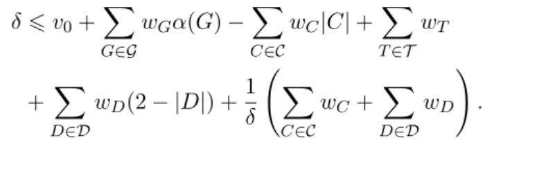
δ6v₀+X

G∈G

w_Gα(G)−X

C∈C

w_C|C|+X

T∈T

w_T

+ X

D∈D

w_D(2− |D|) +1 δ

X

C∈C

w_C+ X

D∈D

w_D

!

.

4. Numerical bounds

Finding the optimal configurations of points for which to invoke constraints (C1) - (c C4) is a tedious task, where we utilized a bootstrap algorithm. Oncec some constraints are fixed, and the corresponding linear program is solved, one has to find numerically a configuration of points for which some of the constraints (C1) - (c C4) is violated. Adding this to the list of constraints, onec again has to execute the above procedure, until no significant improvement is possible to be made this way. At the final step, the large number of graphs and point-sets can be pruned by dropping the non-binding constraints. Our construction in its polished form has 26 linear constraints.

In order to handle the linear program numerically, we discretize it. Based on the previous results, we will only search for the coefficients eκ(ti), where ti = iε0, with ε0 = 0.05 and i 6 12000, thus, ti ∈ [0,600]. For all other values of t>0, we setκ(t) = 0.e

We are going to solve the discretized linear program defined by the fol- lowing graphs and point-sets.

Constraint (C1) -c G family. As in [7], we also found that the optimal graphs to apply (C1) for are suitably positioned copies of thec Moser spindle M, see Figure 1. This unit distance graph has 7 vertices and 11 edges. The optimal locations are so that the origin lies on the axis of symmetry of M, outside the convex hull of M, see Figure 1. The distance of the vertex of M with degree 4 (called theapex ofM) and the origin ranges between 0.55 and 0.85. We apply constraint (C1) to a familyc G of 8 Moser spindles, as described in Table 1.

1

−1

Figure 1. The Moser spindle. All the indicated edges are of unit length.

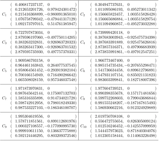
Constraint (C2) -c C point-sets. The optimal C graphs that we found all have 6 vertices. Up to numerical approximations, there are two types of these extremal graphs, see Figure 2. First, take the union of a rhombus of edge length 1 and a segment of length 1 parallel to its longer diagonal, located symmetrically so that the midpoint of the segment lies on the line defined by the shorter diagonal. In the extremal configurations, the distance between the center of the rhombus and the midpoint of the segment is either about 0.9 or about 2.4. The second configuration type is the union of a regular triangle and its translate by a unit vector. The resulting 6-point unit distance graph has 9 edges. Altogether, we use 10 constraints of this type, listed in Table 2.

1

−1

1

1 2

1

−1

Figure 2. The point-sets of familyC

Constraint (C3) -c T triangles. The graphs chosen here are isosceles triangles with the origin lying on their axis of symmetry. The side-lengths of the triangles are either (1,1, a) with a < 1 or (b, b,1) with b ≈ 2. We invoke the constraint for a family T of 5 triangles, three smaller and two bigger ones, presented in Table 3.

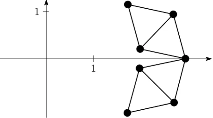
Constraint (C4) -c D graph. Finally, we apply the last constraint to only one graph: Dis a generalized Moser spindle, that is, the union of two rhombi of unit side length and unit shorter diagonal, placed so that they share a common apex, and the distance between the other apices is about 2.24, see Figure 3. Then, Dhas 7 vertices with independence number 3; the coordinates of its vertices are given in Table 4.

1

1

Figure 3. The generalized Moser spindleD.

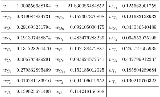
Using these graphs, we construct the witness function W(t) as in Propo- sition 1 with the coefficients described in Table 5. The coefficients arise as the solution of the dual linear program. Because of discretization, the positivity of the function is only guaranteed at the node points. Complete positivity must be checked numerically. We found that the minimum of the function is about −0.0005567, attained at t = 3.82528. Subtracting this minimum value from the original value of v0 leads to the set of coefficients described in Table 5 and to the functionW(t) which satisfies the condition of Proposition 1. Further technical details about the verification are described in [7].

With this construction of W(t), the quadratic equation (15) takes the form

δ²+ 8.412286934947δ−2.226873241160 = 0, whose positive solution is δ= 0.256873013577.

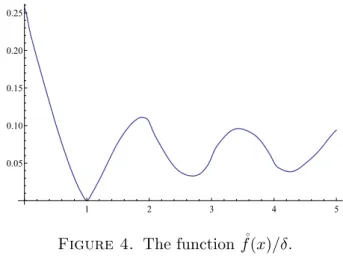
The coefficients eκ(t) obtained as the solution of the linear program (13) also provide the normalized, radialized autocorrelation function ˚f(x) via (8) and (12). This function is plotted on Figure 4.

1 2 3 4 5

0.05 0.10 0.15 0.20 0.25

Figure 4. The function ˚f(x)/δ.

5. Appendix: Numerical values

G₁ 0.549394809875 G₂ 0.574818438480 G₃ 0.589129645929 G₄ 0.730924687690 G₅ 0.745526562977 G₆ 0.810398355949 G₇ 0.821514458830 G₈ 0.844783781915

Table 1. The familyGof the copies of Moser spindles, which are located so that the origin lies on the axis of symmetry, outside the convex hull. The norm of the apex is listed.

( 0.406817237137, 0 ) ( 0.304947737631, 0 ) ( 0.212653201726, 0.979424301472) ( 1.011095086193, 0.495273011342) C1 ( 0.215416368899,−0.980091365010) C2 ( 0.156665823457, 1.003515826428) ( 1.076758799342,−0.479441317129) ( 0.156665686884,−1.003515829754) ( 1.092173797015, 0.514761385947) ( 1.011094960857,−0.495273032288)

( 0.722707873034, 0 ) ( 0.739999420118, 0 )

( 2.879596197060,−0.497750114205) ( 0.387683003943,−0.925475734398) C3 ( 0.383263232831, 0.926963720323) C4 ( 0.387683391889, 0.925475626816) ( 0.383263417300,−0.926963701532) ( 2.873857316371, 0.497906683939) ( 2.879595735930, 0.497757370331) ( 2.873855991861,−0.497912547251)

( 1.909586793158, 0 ) ( 1.966773467400, 0 )

( 0.964461163843, 0.264077537545) ( 0.985154735434,−0.207655298471) C₅ ( 0.958064561452,−0.293919382104) C₆ ( 1.541736634458, 0.899612796891) ( 0.700166154949, 0.716490286642) ( 0.547931107154, 0.835021131823) ( 1.665508028159, 0.957346037548) ( 0.983603399841, 0.182718007396)

( 1.971873970831, 0 ) ( 1.977604739521, 0 )

( 0.987645642144, 0.175007132703) ( 0.990398355678, 0.157171481656) C7 ( 1.585316335898, 0.914734021728) C8 ( 0.599752268603, 0.799043686844) ( 0.598742912958, 0.798018249330) ( 0.991555248207,−0.187167815493) ( 0.987533227103,−0.186346100707) ( 1.586930662216, 0.912324929889)

( 1.995304619556, 0 ) ( 2.019750708108, 0 )

( 1.578711851561, 0.899112691976) ( 0.556472755654, 0.826305009124) C₉ ( 1.000327108557,−0.177090995730) C₁₀ ( 1.012516246452,−0.142557099959) ( 0.999910611150, 0.136637775888) ( 1.544457973623, 0.871840304076) ( 0.592124446295, 0.803209372546) ( 1.012305158444, 0.114063226498)

Table 2. Collection C of point-sets used. Each of the sets also contains the origin (0,0), so each set has 6 points.

(−0.726108320018, 0 ) (−0.746389938122, 0 )

T₁ ( 0.155933903426,−0.381702431017) T₂ ( 0.151459324640, 0.350598185034) ( 0.155933903426, 0.381702431017) ( 0.151459324640,−0.350598185034)

(−0.799108011229, 0 ) (−0.122154919695, 0 )

T3 ( 0.110687746283, 0.328281974673) T4 ( 1.939660687516, 0.500789551558) ( 0.110687746283,−0.328281974673) ( 1.939660687516,−0.500789551558)

(−0.133851861793, 0 )

T₅ ( 1.934710898446, 0.500150467476) ( 1.934710898446,−0.500150467476)

Table 3. The family T of triangles used for the estimates.

(2.929162925441, 0 ) (2.590194413036, 0.940797718746) (1.944923944982, 0.176843516547) D (1.605955432577, 1.117641235293) (2.590194413036,−0.940797718746) (1.944923944982,−0.176843516547) (1.605955432577,−1.117641235293)

Table 4. The graphD, a generalized Moser spindle.

v₀ 1.000556688164 v₁ 21.830086484852 w_G1 0.125663001758 w_G2 0.319084834731 w_G3 0.152397370898 w_G4 0.121683128933 w_G5 0.291693251794 w_G6 0.092105000475 w_G7 0.343036540489 w_G8 0.191307438874 w_C1 0.483479288239 w_C2 0.064553075196 w_C3 0.131728260470 w_C4 0.192138472887 w_C5 0.265727605935 wC6 0.006785989291 wC7 0.093924572541 wC8 0.442799912237 wC9 0.279332895469 wC10 0.152185012025 wT1 0.185804289684 wT2 0.010281183916 wT3 0.094109619652 wT4 0.130215766322 wT5 0.139825671498 wD 0.114218156868

Table 5. Coefficients of the witness functionW(t) of Propo- sition 1.

References

[1] C. Bachoc, A. Passuello, and A. Thiery, The density of sets avoiding distance 1 in Euclidean space. Discrete & Computational Geometry53(2015), 783-808.

[2] H. T. Croft,Incidence incidents. Eureka30(1967), 22–26.

[3] E. DeCorte, F. M. de Oliveira Filho, and F. Vallentin, Complete positivity and distance-avoiding sets.arXiv:1804.0909 (2018), 1–58.

[4] P. Erd˝os,Problems and results in combinatorial geometry.in: Discrete Geometry and Convexity (New York, 1982), Annals of the New York Academy of Sciences440, New York Academy of Sciences, New York, 1985, pp. 1-11.

[5] A. de Grey,The chromatic number of the plane is at least 5. arXiv:1804.02385 (2018).

[6] Y. Katznelson,An introduction to Harmonic Analysis.Wiley, New York, 1968.

[7] T. Keleti, M. Matolcsi, F. M. de Oliveira Filho, and I. Z. Ruzsa,Better bounds for planar sets avoiding unit distances.Discrete & Computational Geometry55(2016), 642-661.

[8] L. Moser, W. Moser,Solution to problem 10.Canadian Math. Bull.4(1961), 187–189.

[9] F. M. de Oliveira Filho and F. Vallentin,Fourier analysis, linear programming, and densities of distance-avoiding sets inRⁿ. Journal of the European Mathematical So- ciety12(2010), 1417–1428.

[10] L. A. Sz´ekely,Erd˝os on unit distances and the Szemer´edi-Trotter theorems. in: Paul Erd˝os and His Mathematics II (G. Hal´asz, L. Lov´asz, M. Simonovits, and V. T. S´os, eds.), Bolyai Society Mathematical Studies11, J´anos Bolyai Mathematical Society, Budapest; Springer- Verlag, Berlin, 2002, pp. 646–666.

Gergely Ambrus, Alfr´ed R´enyi Institute of Mathematics, Hungarian Acad- emy of Sciences, POB 127 H-1364 Budapest, Hungary.

E-mail address: ambrus@renyi.hu

M´at´e Matolcsi: Budapest University of Technology and Economics (BME), H-1111, Egry J. u. 1, Budapest, Hungary (also at Alfr´ed R´enyi Institute of Mathematics, Hungarian Academy of Sciences, POB 127 H-1364 Budapest, Hungary).

E-mail address: matomate@renyi.hu