https://doi.org/10.1007/s10878-020-00655-4
The maximum Wiener index of maximal planar graphs
Debarun Ghosh1·Ervin Gy ˝ori1,2·Addisu Paulos1,3·Nika Salia1,2 · Oscar Zamora1,4
Accepted: 22 September 2020
© The Author(s) 2020
Abstract
The Wiener index of a connected graph is the sum of the distances between all pairs of vertices in the graph. It was conjectured that the Wiener index of ann-vertex maximal planar graph is at most181(n3+3n2). We prove this conjecture and determine the uniquen-vertex maximal planar graph attaining this maximum, for everyn≥10.
Keywords Wiener index·Planar graphs·Triangulation·Distance·Mini–Max
1 Introduction
The Wiener index is a graph invariant based on distances in the graph. For a connected graph G, the Wiener index is the sum of distances between all unordered pairs of vertices in the graph and is denoted byW(G). That means,
W(G)=
{u,v}⊆V(G)
dG(u, v).
B
Nika Saliasalia.nika@renyi.hu Debarun Ghosh
ghosh_debarun@phd.ceu.edu Ervin Gy˝ori
gyori.ervin@renyi.hu Addisu Paulos
paulos_addisu@phd.ceu.edu Oscar Zamora
zamora-luna_oscar@phd.ceu.edu
1 Central European University, Budapest, Hungary 2 Alfréd Rényi Institute of Mathematics, Budapest, Hungary 3 Addis Ababa University, Addis Ababa, Ethiopia 4 Universidad de Costa Rica, San José, Costa Rica
wheredG(u, v)denotes the distance fromu tov i.e. the minimum length of a path fromutovin the graphG.
It was first introduced by Wiener (1947) while studying its correlations with boiling points of paraffin considering its molecular structure. Since then, it has been one of the most frequently used topological indices in chemistry, as molecular structures are usually modelled as undirected graphs. Many results on the Wiener index and closely related parameters such as the gross status (Harary 1959), the distance of graphs (Entringer et al.1976), and the transmission (Šoltés1991) have been studied.
A great deal of knowledge on the Wiener index is accumulated in several survey papers (Dobrynin et al.2001,2002; Dobrynin Mel’nikov2012; Knor and Škrekovski2014;
Xu et al.2014). Finding a sharp bound on the Wiener index for graphs under some constraints has been one of the research topics attracting many researchers.
The most basic upper bound ofW(G)states that, ifGis a connected graph of order n, then
W(G)≤ (n−1)n(n+1)
6 , (1)
which is attained only by a path (Dankelmann et al.2008a; Plesník1984; Lovász 1979). Many sharp or asymptotically sharp bounds onW(G)in terms of other graph parameters are known, for instance, minimum degree (Beezer et al.2001; Dankel- mann and Entringer 2000; Kouider and Winkler1997), connectivity (Dankelmann et al.2009; Favaron et al.1989), edge-connectivity (Dankelmann et al.2008b,a) and maximum degree (Fischermann et al.2002). For finding more details in mathemat- ical aspect of Wiener index, see also results (Das and Nadjafi-Arani2017; Gutman et al.2014; Klavžar and Nadjafi-Arani2014; Knor et al.2014, 2016; Li et al.2018;
Mukwembi and Vetrík2014; Wagner et al.2009; Wagner2006; Wang and Yu2006).
One can study the Wiener index of the family of connected planar graphs. Since the bound given in Eq.1is attained by a path, it is natural to ask the same question for some particular family of planar graphs. For instance, the Wiener index of a maximal planar graph withnvertices,n≥3 has a sharp lower bound(n−2)2+2. This bound is attained by any maximal planar graph such that the distance between any pair of vertices is at most 2 (for instance a planar graph containing then-vertex star). Che and Collins (2018), and independently ´Czabarka et al. (2019), gave a sharp upper bound of a particular class of maximal planar graphs known asApollonian networks. An Apollonian network may be formed, starting from a single triangle embedded on the plane, by repeatedly selecting a triangular face of the embedding, adding a new vertex inside the face, and connecting the new vertex to each of the three vertices of the face.
They showed that
Theorem 1.1 (Che and Collins2018; ´Czabarka et al.2019)Let G be an Apollonian network of order n≥3. Then W(G)has a sharp upper bound
W(G)≤ 1
18(n3+3n2)
=
⎧⎪
⎨
⎪⎩
1
18(n3+3n2), if n≡0(mod3);
1
18(n3+3n2−4), if n≡1(mod3);
1
18(n3+3n2−2), if n≡2(mod3).
It has been shown explicitly in Che and Collins (2018) that the bound is attained for the maximal planar graphs Tn, we will give the construction of Tn in the next section, see Definition2.1. The authors in Che and Collins (2018) also conjectured that this bound also holds for every maximal planar graph. It has been shown that the conjectured bound holds asymptotically ( ´Czabarka et al.2019). In particular, they showed the following result.
Theorem 1.2 ( ´Czabarka et al. (2019))For k=3,4,5, there exists a constant Cksuch that
W(G)≤ 1
6kn3+Ckn5/2 for every k-connected maximal planar graph of order n.
In this paper, we confirm the conjecture.
Theorem 1.3 Let G be an n≥6vertex maximal planar graph. Then
W(G)≤ 1
18(n3+3n2)
=
⎧⎪
⎨
⎪⎩
1
18(n3+3n2), if n≡0(mod3);
1
18(n3+3n2−4), if n≡1(mod3);
1
18(n3+3n2−2), if n≡2(mod3).
Equality holds if and only if G is isomorphic to Tnfor all n≥9.
2 Notations and preliminaries
LetGbe a graph. We denote vertex set and edge set ofGbyV(G)andE(G)respec- tively. A path in a graph is an alternating sequence of distinct vertices and edges, starting from a vertex and ending at a vertex. Such that every edge is incident to neigh- bouring vertices in the sequence. The length of the path is the number of edges in the given path. With a slight abuse of notion, a cycle in a graphGis a non-zero length path from a vertexvto itselfv. We use standard functiondG(v,u)to denote the length of shortest path from the vertexvto the vertexu. Even more, we may define a function that denotes the distance from a vertex to the set of vertices. Letvbe a vertex ofG andS⊆V(G)thendG(S, v):=mi nu∈S{dG(u, v)}.
For a vertex setS ⊂ V(G), thestatusofS is defined as the sum of all distances from the vertices of the graph to the setS. It is denoted byσG(S), thus
σG(S):=
u∈V(G)
dG(S,u).
For simplicity, we may omit subscriptGin the given functions if the underlined graph is obvious. With a slight abuse of notation, we useσG(v):=σG({v}).
We have,
W(G)=1 2
v∈V(G)
σG(v).
|n |(n−1)
(a)3 (b)3 (c)3|(n−2)
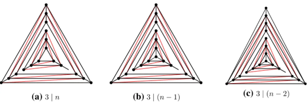
Fig. 1 Apollonian networks maximizing Wiener index of maximal planar graphs, Che and Collins (2018)
Here we use definition from Che and Collins (2018), for an Apollonian network Tnonnvertices. We will prove later that it is the unique maximal planar graph that maximizes the Wiener index of the maximal planar graphs.
Definition 2.1 (Che and Collins (2018)) The Apollonian networkTn is the maximal planar graph onn≥3 vertices, with the following structure, see Fig.1.
Ifnis a multiple of 3, then the vertex set ofTncan be partitioned in three sets of same size,A= {a1,a2,· · · ,ak},B = {b1,b2, . . . ,bk}andC= {c1,c2,· · ·,ck}. The edge set ofTn is the union of following three setsE1 = ki=1{(ai,bi), (bi,ci), (ci,ai)}
forming concentric triangles, E2 = ki=−11{(ai,bi+1), (ai,ci+1), (bi,ci+1)}forming
‘diagonal’ edges, and E3= k1−1{(ai,ai+1), (bi,bi+1), (ci,ci+1)}forming paths in each vertex class, see Fig.1a.
If 3|(n−1), thenTnis the Apollonian network which may be obtained fromTn−1
by adding a degree three vertex in the facea1,b1,c1oran−1 3 ,bn−1
3 ,cn−1
3 , see Fig.1b.
Note that both graphs are isomorphic.
If 3|(n−2), thenTnis the Apollonian network which may be obtained fromTn−2
by adding a degree three vertex in each of the facesa1,b1,c1andan−1 3 ,bn−1
3 ,cn−1 3 , see Fig.1c.
The following lemmas will be used in the proof of Theorem1.3. At first, we would like to recall some standard definitions. A connected graph Gis said to besvertex connected or simply s-connectedif it has more thansvertices and remains connected whenever fewer thans vertices are removed. An induced subgraph of a graphGis another graph, formed from a subset of the vertices ofGand all of the edges connecting pairs of vertices in that subset. Formally letGbe a graph andSbe a subset of vertices of G,S ⊆V(G). Then induced subgraphG[S]ofGis a graph on the vertex setSand and E(G[S])= {e∈ E(G):e⊆S}. A connected graphGis calledHamiltonian graph, if there is a cycle that includes every vertex of G, and the cycle is calledHamiltonian cycle.
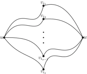
Lemma 2.2 Let G be an s-connected, maximal planar graph and S be a cut set of size s of G. Then G[S]is Hamiltonian.
Proof Let us denote vertices ofS,S = {v1, v2, . . . , vs}. Letuandwbe two distinct vertices,{u, w} ∈V(G)\Ssuch that any path fromutowcontains at least one vertex
Fig. 2 spairwise disjoint paths fromutow
u w
v
i1v
i2v
is−1v
isfromS. SinceGiss-connected, by Menger’s Theorem, there arespairwise internally vertex disjoint paths fromutow. Each of the paths intersectsSin disjoint nonempty sets, therefore each of the paths contains exactly one vertex fromS. We may assume, that in a particular planar embedding ofG, those paths are ordered in such a way that one of the two regions determined by the cycle obtained from two paths fromu to wcontainingvix andvix+1 has no vertex fromS(where indices are taken modulos), see Fig.2. From the maximality of the planar graph, there is a path from the vertexu to the vertexwthat does not contain a vertex fromS, a contradiction. Thus we must have the edges{vix, vix+1}. Therefore we have a cycle of lengthson the vertex setS, vi1, vi2,· · ·, vis, vi1 in the given order. henceG[S]is Hamiltonian.
The following definition is particularly helpful for the proof of Theorem1.3. Given a set S ⊆ V, we define the Breadth First Search partition ofV with root S,PSG or simplyPSwhen the underline graph is clear, byPS= {S0,S1, . . .}, whereS0 =S, and fori≥1,Si is the set of vertices at distance exactlyifromS, formallySi = {v∈ V(G): dG(S, v)=i}. We refer to those sets aslevelsofPs. In particularS1is the first level. For the largest integer integerk, for whichSk= ∅, we refer toSkas thelast level. We refer toS0and the last level asterminal level. Note that by definition every level besides the terminal level is a cut set ofG. We denote byPvthe Breadth First Search partition from{v}, that is the partitionP{v}.
The following three lemmas play a critical role to prove Theorem1.3.
Lemma 2.3 Let G be an n+s vertex graph and S, S⊂V(G), be a set of vertices of size s. Such that each non-terminal level ofPShas size at least3. Then we have
σ(S)≤σ3(n):=
1
6(n2+3n), if n≡0(mod3);
1
6(n2+3n+2), if n≡1,2(mod3).
Proof. IfPS= {S0,S1, . . .}, by definition, we have thatσ (S)=
i
i|S|.Therefore
σ (S)= |S1| +2|S2| +3|S3| + · · ·
≤3
1+2+ · · · +n
3 + n
3 +1
n−3
n
3 =σ3(n).
Lemma 2.4 Let G be an n+s vertex graph and S, S⊂V(G), be a set of vertices of size s. Such that each non-terminal level ofPShas size at least4. Then we have
σ(S)≤σ4(n):=
⎧⎪
⎨
⎪⎩
1
8(n2+4n), if n≡0(mod4);
1
8(n2+4n+3), if n≡1,3(mod4);
1
8(n2+4n+4), if n≡2(mod4).
Proof. We have σ (S)≤4
1+2+ · · · + n−1
4 + n−1
4
+1
n−1−4 n−1
4
=σ4(n)
Lemma 2.5 Let G be an n+s vertex graph and S, S⊂V(G), be a set of vertices of size s. Such that each non-terminal level ofPShas size at least5. Then we have
σ(S)≤σ5(n):=
⎧⎪
⎨
⎪⎩
1
10(n2+5n), if n≡0(mod5);
1
10(n2+5n+4), if n≡1,4(mod5);
1
10(n2+5n+6), if n≡2,3(mod5).
Proof. We have σ (S)≤5
1+2+ · · · + n−1
5 + n−1
5
+1
n−1−5 n−1
5
=σ5(n)
3 Proof of Theorem1.3
Proof From Che and Collins (2018), we know that the desired lower bound is attained for Tn. For the upper bound, we are going to prove Theorem 1.3by induction on the number of vertices. In Che and Collins (2018), they prove it forn ≤10 without computer aid, but in ´Czabarka et al. (2019), it is shown that the upper bound of Theorem 1.3holds, for 6≤n ≤ 18 with using computer program. It is also shown by means of computer program that the upper bound is sharp for 6≤n ≤18 and the extremal graph is uniqueTnfor 9≤n≤18. For our proof, we use the computer-aided result of Czabarka et al. (2019) only for Case 2.1 and for the uniqueness of the extremal graph.´
For the rest, the result in Che and Collins (2018) is enough. Unfortunately, we do not know any proof of the casesn ≤ 18 without the use of computers. So, we assume n≥19 from now on.
LetGbe a maximal planar graph ofn≥19 vertices. The proof contains three cases depending on the connectivity of the graphG. SinceGis a maximal planar graph, it is either 3, 4 or 5-connected. Notice that the result in ´Czabarka et al. (2019) is much stronger asymptotically than ours ifGis 4 or 5-connected, but we are to prove the upper bound for everyn ≥19. In Case 2, it makes the proof somewhat technical.
Case 1LetGbe a 5-connected graph. For every fixed vertexv∈V(G), considerPv. SinceGis 5-connected, and each of the non-terminal levels ofPvis a cut set, we have that each non-terminal level has size at least 5. Therefore from Lemma2.5, we have,
W(G)= 1 2
v∈V(G)
σ(v)≤ n
2σ5(n−1)≤ n
20(n2+3n+2) <
1
18(n3+3n2)
,
for alln≥4. Therefore we are done ifGis 5-connected.
Case 2LetGbe 4-connected and not 5-connected. ThenGcontains a cut set of size 4, which induces a cycle of length four, by Lemma2.2. Let us denote the vertices of this cut set asv1, v2, v3andv4, forming the cycle in this given order. The cut-set divides the plane into two regions. We call them the inner and the outer region respectively.
Let us denote the number of vertices in the inner region byxand assume, without loss of generality, thatxis minimal possible, but greater than one. Obviouslyx≤ n−24 or x=n−5. From here on, we deal with several sub-cases depending on the value ofx.
Case 2.1Ifx≥4 andx=n−5.
Let us consider the sub-graph ofG, sayG, obtained by deleting all vertices from the outer region of the cyclev1, v2, v3, v4inG. The graphG is not maximal since the outer face is a 4-cycle. The graphGis 4-connected, therefore it does not contain neither{v1, v3}nor{v2, v4}, consequently we may add any of them toG, to obtain a maximal planar graph. Adding an edge decreases the Wiener index ofG. In the following paragraph, we prove that one of the edges decreases the Wiener index ofG by at most x162.
Let Ai = {v ∈ V(G)|d(v, vi) < d(v, vj),∀j ∈ {1,2,3,4}\{i}} for i ∈ {1,2,3,4}. Let Abe the subset of vertices of G not contained in any of the Ai’s.
So A,A1,A2,A3,A4is a partition of vertices ofG. It is simple to observe that, if adding an edge {vi, vi+2}, for i ∈ {1,2}, decreases the distance between a pair of vertices, then these vertices are from Ai andAi+2. If there is a vertexuwhich has at least three neighbours from the cut set, without loss of generality sayv1, v2, v3, then A2 = ∅, sinceGis 4-connected. Therefore we are done if there exists such vertex.
Otherwise, for each pair{v1, v2},{v2, v3},{v3, v4},{v4, v1}, there is a distinct vertex which is adjacent to both vertices of the pair. Hence the size of Ais at least 4. The size of the vertex set∪4i=1Ai, is at mostx. By the AM-GM inequality, we have that one of|A1| · |A3| or|A2| · |A4|is at most x162. Therefore we can choose one of the edges{v1, v3}or{v2, v4}, such that after adding that edge to the graphG, the Wiener index of the graph decreases by at most x162. Let us denote the maximal planar graph obtained by adding this edge toGbyGx+4.
Similarly, we denote the maximal planar graph obtained fromG, by deleting all vertices in the inner region and adding the diagonal by Gn−x. This decreases the Wiener index by at most (n−x16−4)2.
Consider the graphGn−x and a sub-set of it’s verticesS = {v1, v2, v3, v4}. Since the graphGis 4-connected, each non-terminal level ofPSGn−x has at least 4 vertices.
Therefore we get thatσGn−x(S)≤σ4(n−x−4)=(n−x8−2)2, from Lemma2.4.
Recall thatGis the graph obtained fromGby deleting the vertices from the outer region. For eachi ∈ {1,2,3,4}, consider the BFS partitionPvGi. Note that,x ≥ 4, G is 4-connected, and by minimality ofx, we have that every non-terminal level of PvGi has at least 5 vertices, except two cases. The first level may contain only four vertices and the penultimate level may also contain four vertices with the last level having exactly one vertex. Status of thevi is maximised, if the number of vertices in the first and the penultimate level is four, with the last level containing only one vertex and every other level contains exactly five vertices.
To simplify calculations of the status of the vertexvi, we may hang a new temporary vertex on the root, and we may bring a vertex from the last level to the previous level.
These modifications do not change the status of the vertex, but it increases the number of vertices. Now we may apply Lemma2.5for this BFS partition, considering that num- ber of vertices in all levels is exactly 5. Therefore we haveσG(vi)≤ (x+4)210+5(x+4). Observe that this status contains distances, fromvi to other vertices from the cut set, which equals to four. Note that this is a uniform upper bound for the status of each of the vertices from the cut set.
Finally we may upper bound the Wiener index ofGin the following way,
W(G)≤W(Gn−x)+(n−x−4)2
16 +W(Gx+4)+ x2 16−8
+x·σGn−x({v1, v2, v3, v4})+(n−x−4)·(σG(v1)−4).
In the first line, we upper bound all distances between pairs of vertices on the cut set and outer region, and between pairs of vertices on the cut set and inner region. We subtract 8 since distances between the pairs from the cut set were double-counted. In the second line, we upper bound all distances from the outer region to the inner region.
These distances are split in two, distances from the outer region to the cut set and from a fixed vertex of the cycle, without loss of generality sayv1, to the inner region.
We are going to prove thatW(G)≤ 181(n3+3n2)−1, therefore we will be done in this sub-case. We need to prove the following inequality
1
18(n3+3n2)−1≥ 1
18((n−x)3+3(n−x)2)+(n−x−4)2 16 + 1
18((x+4)3+3(x+4)2)+x2 16−8 +x·(n−x−2)2
8 +(n−x−4)·((x+4)2+5(x+4)
10 −4).
After we simplify, we get 82
45−9n 10+n2
16+x
5 +41nx 120 −n2x
24 −3x2 40 +nx2
60 +x3
40 ≤0. (2)
We know that 4 ≤ x ≤ n−24 and if we setx =4, we get 2176+528n−75n2 ≤ 0 which holds for all≥ 10. Therefore, if the derivative of the right hand side of the inequality is negative for all{x |4≤x≤ n−24}, then the inequality holds for all these values ofx. Differentiating the LHS of the Inequality (2), with respect tox, we get
δ δx
82 45−9n
10 +n2 16+ x
5 +41nx 120 −n2x
24 −3x2 40 +nx2
60 +x3 40
=1 5 +41n
120 −n2 24−3x
20 +nx 30 +3x2
40 .
(3)
If we setx =4 in Eq.3, we get 1201 (96+57n−5n2), which is negative for all
≥ 13. If we setx = n−24 in Eq.3, we get 1601 (−n2+8n+128), which is negative for all≥17. Therefore Eq.3is negative in the whole interval. Sincen≥19, we have W(G)≤ 181(n3+3n2)−1, and this sub-case is settled.
Case 2.2If 2≤x≤3.
From the minimality ofx and maximality ofG, we havex = 2. Let us consider the maximal planar graph, denoted byGn−2, obtained fromGby deleting these two vertices from the inner region and adding an edge which decreases the Wiener index by at most (n−166)2, such edge exists as in the previous case.
SinceGis 4-connected, for each vertexv,v ∈ V(G), each level ofPvG contains at least 4 vertices, but possibly the last one. Therefore status of both vertices inside can be bounded byσ5(n)= 18((n−1)2+4(n −1)+4). This bound comes from Lemma2.4. Finally, we have
W(G)≤W(Gn−2)+(n−6)2
16 +2
8((n−1)2+4(n−1)+4)−1
≤ 1
18((n−2)3+3(n−2)2)+(n−6)2
16 +2
8((n−1)2+4(n−1)+4)−1
= 1
18n3+ 7 48n2−1
4n+49
18−1≤ 1
18(n3+3n2)−1.
(4) The last inequality holds for alln≥9, so this sub-case is done too.
Case 2.3Ifx=n−5.
Therefore we have one vertex outside of the cut set. Let us consider the maximal planar graph, denoted byGn−1, obtained fromGby deleting the vertex from the outer region and adding an edge which decreases the Wiener index by at most(n−165)2.
By the choice ofx, we have that for the vertex outside the cut setv. Each level ofPvG contains at least 5 vertices, except the first one which contains only 4 and the penultimate level may contain 4 vertices too followed by one vertex in the last level.
The status of the vertexvis maximized if the last level contains exactly one vertex, the penultimate and the first level contain four vertices while every other level contains five vertices. Therefore status ofvcan be bounded by101(n2+5n). This bound comes from Lemma2.5. Finally, we have
W(G)≤W(Gn−1)+(n−5)2
16 + 1
10(n2+5n)
≤ 1
18((n−1)3+3(n−1)2)+(n−5)2
16 + 1
10(n2+5n)
= 1
18n3+13 80n2+ 7
24n−241 144 ≤ 1
18(n3+3n2)−1.
(5)
The last inequality holds for alln≥9, so this sub-case is done too.
Case3. LetGbe 3-connected and not 4-connected. SinceGis not 4-connected and it is a maximal planar graph, it must have a cut set of size 3, say{v1, v2, v3}. This induces a triangle from the Lemma2.2. Without loss of generality, let us assume that number of vertices in the inner smaller region of the cut set is minimal possible, say x.
Case3.1.Ifx≤2.
From the minimality of x, we have x = 1. Let us denote this vertex asv. Let Gn−1be a maximal planar graph obtained fromGby deleting the vertexv. From the Lemma2.3, we haveσG(v)≤ 16(n2+n)−1313|(n−1), where13|(n−1)equals one if 3 dividesn−1 and zero otherwise. Finally we have,
W(G)≤W(Gn−1)+σG(v)
≤ 1
18((n−1)3+3(n−1)2)−1
913|n−2
913|(n−2)+1
6(n2+n)
−1
313|(n−1)= n3 18+n2
6 +1 9 −1
913|(n)−2
913|(n−2)−1 313|(n−1)
≤ 1
18(n3+3n2)
.
(6)
In this case, the equality holds if and only if the graph obtained after deleting the vertex visTn−1. We can observe that, if we add the vertexvto the graphTn−1, the choice that maximizes the status ofv,σG(v)= 16(n2+n)−1313|(n−1), is only when we add vin one ot the two faces which gets us the graphTn. Hence we have the desired upper bound of the Wiener index and equality holds if and only ifG=Tn.
Case 3.2Ifx=3.
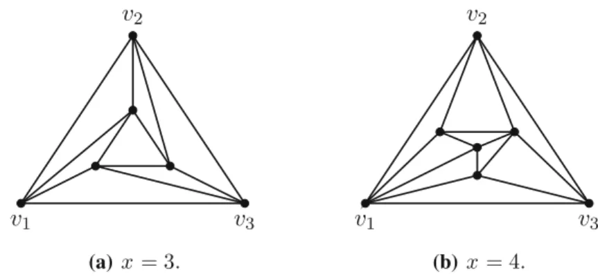
Let us denote vertices in the inner region as x1, x2andx3. From the minimality ofxand maximality ofG, the structure ofGin the inner region is well defined, see Fig.3a. If we remove these three inner vertices, the graph we get is denoted byGn−3
and is still maximal. Hence we may use the induction hypothesis for the graphGn−3. Consider the graphGn−3and a vertex setS= {v1, v2, v3}. Each level ofPSGn−3has at least three vertices except the terminal one. Therefore we may apply Lemma2.3, then we haveσGn−3({v1, v2, v3})≤ 16((n−6)2+3(n−6)+2). To estimate distances from the vertices in the outer region to the vertices in the inner region we do the following.
v
1v
3v
2(a)x = 3.
v
1v
3v
2(b) x = 4.
Fig. 3 The unique inner regions for the 3-connected case whenx=3 andx=4
We first estimate distances from the outer region to the cut set and from the fixed vertex on the cut set to allxi. The distances from the vertices in the outer region to the set{v1, v2, v3}, isσGn−3({v1, v2, v3}). The sum of distances fromvito the vertices {x1,x2,x3}is 4. Note that, if we take a vertex in the outer region which has at least two neighbours on the cut set, then for this vertex we need to count 3 for the distances from the cut set to the vertices{x1,x2,x3}. Since we have at least two such vertices, all cross distances can be bounded by 3σGn−3({v1, v2, v3})+4(n−5)+6. Then we have,
W(G)≤W(Gn−3)+W(K3)+3σGn−3({v1, v2, v3})+4n−14
≤ 1
18((n−3)3+3(n−3)2)+1
2((n−6)2+3(n−6)+2)+4n−11
<
1
18(n3+3n2)
. (7)
Therefore, this case is also settled.
Case 3.3Ifx=4.
From the minimality ofxand the maximality of the planar graphG, there is only one configuration of the inner region (Fig.3b). Consider a maximal planar graph on the n−4 vertices, sayGn−4, that is obtained fromGby deleting the four inner vertices. We will apply the induction hypothesis for this graph, to upper bound the sum of distances between all pairs of vertices fromV(Gn−4)inG. By applying Lemma2.3forGn−4
andS= {v1, v2, v3}, we getσGn−4({v1, v2, v3})≤ 16((n−4−3)2+(n−4−3)+2). The sum of the distances between the four inner vertices is 7. The sum of the distances from eachvi to all of the vertices inside is at most six. By a similar argument as in the previous case we have,
W(G)≤ 1
18((n−4)3+3(n−4)2)+7+4
6((n−7)2+(n−7)+2)+6(n−4)
<
1
18(n3+3n2)
. (8)
v1 v3
v2
v1 v3
v2
v1 v3
v2
Fig. 4 3-Connected,x=5
Therefore, this case is also settled.
Case 3.4Ifx=5.
From the minimality ofxand the maximality of the planar graphG, there are three configurations of the inner region, see Fig.4. Consider a maximal planar graph on the n−5 vertices, sayGn−5, which is obtained fromGby deleting 5 vertices from the inner region. We will apply the induction hypothesis for this graphGn−5, to bound the sum of the distances between the vertices ofV(Gn−5)in the graphG. By applying Lemma2.3 forGn−5andS= {v1, v2, v3}, we getσGn−5({v1, v2, v3})≤ 16((n−8)2+(n−8)+2).
The sum of the distances between five inner vertices is at most 13. The sum of the distances fromvito all of the vertices inside is at most 8. Finally, we have
W(G)≤ 1
18((n−5)3+3(n−5)2)+13+5
6((n−8)2+(n−8)+2)+8(n−5)
<
1
18(n3+3n2)
. (9)
Therefore this case is also settled.
Case 3.5Ifx≥6.
First we settle forx ≥7 and then forx =6. Consider the maximal planar graph onn−xvertices, sayGn−x, which is obtained fromGby deleting thosexvertices from the inner region of the cut set{v1, v2, v3}. Consider the maximal planar graph onx+3 vertices, sayGx+3, which is obtained fromG, by deleting alln −x−3 vertices from the outer region of the cut set{v1, v2, v3}. We know by induction that W(Gx+3) ≤ 181((x+3)3+3(x+3)2). There are at least two vertices from the cut set{v1, v2, v3}, such that each of them has at least two neighbours in the outer region of the cut set. Without loss of generality, we may assume they arev1andv2. Hence if we consider PvG1n−x and PvG2n−x, we will have 4 vertices in the first level of and at least three in the following levels until the last one. Therefore we have σGn−x(v1)≤σ3(n−x−2)+1≤ 16((n−x−2)2+3(n−x−2)+8)from Lemma2.3 and same forv2. Now let us considerP{vG1x,v+32}, from minimality ofx, each non-terminal level of theP{vG1x,v+32}contains at least 4 vertices. Therefore by applying Lemma2.4, we
getσGx+3({v1, v2})≤ 18(x2+6x+9). We have,
W(G)≤(W(Gx+3)+W(Gn−x)−3)+(n−x−3)(σGx+3({v1, v2})−1) +x
max
σGn−x(v1), σGn−x(v2)
−2
. (10)
The first term of the sum is an upper bound for the sum of all distances which does not cross the cut set. The second and the third terms upper-bounds all cross distances in the following way- we may split this sum into two parts for each crossing pair sum from inside to the set{v1, v2}and fromvi,i ∈ {1,2}to the vertex outside, those are the second and the third terms of the sum accordingly. Therefore applying estimates, we get
1
18(n3+3n2)−1≥ 1
18((x+3)3+3(x+3)2)+ 1
18((n−x)3+3(n−x)2)−3 +(n−x−3)(x2+6x+1)
8
+x((n−x−2)2+3(n−x−2)−4)
6 .
(11) After simplification we have
−x3+x2(n+3)+x(21−6n)−(15+3n)≥0. (12) where
δ δx
−x3+x2(n+3)+x(21−6n)−(15+3n)
= −3x2+(2n+6)x+21−6n. The derivative is positive whenx∈ [7,n2]. Hence since the inequality (12) holds for x=7, it also holds for allx,x ∈ [7,n2]. Therefore, ifx≥7 we are done.
Finally ifx =6, then distances fromv1andv2 to all vertices inside is 9 instead of 738 as it was used the in Inequality11. Thus we get an improvement of Inequality (11), which shows thatW(G) <1
18(n3+3n2)
even forx=6. Therefore we have settled 3-connected case too.
4 Concluding remarks
There is the unique maximal planar graphTn, maximizing the Wiener index, Theo- rem1.3. ClearlyTnis not 4-connected. One may ask for the maximum Wiener index for the family of 4-connected and 5-connected maximal planar graphs. In ´Czabarka et al. (2019), asymptotic results were proved for both cases. Moreover, based on their constructions, they conjecture sharp bounds for both 4-connected and 5-connected maximal planar graphs. Their conjectures are the following.
Conjectute 4.1 LetGbe ann ≥6 vertex maximal 4-connected planar graph. Then
W(G)≤
⎧⎪
⎨
⎪⎩
1
24n3+14n2+13n−2, ifn≡0,2(mod4);
1
24n3+14n2+245n−32, ifn≡1(mod4);
1
24n3+14n2+245n−1, ifn≡3(mod4);
Conjectute 4.2 LetGbe ann ≥12 vertex maximal 4-connected planar graph. Then
W(G)≤
⎧⎪
⎪⎪
⎪⎪
⎪⎨
⎪⎪
⎪⎪
⎪⎪
⎩
1
30n3+103n2−2315n+32, ifn≡0(mod5);
1
30n3+103n2−2315n+1565 , ifn≡1(mod5);
1
30n3+103n2−2315n+1685 , ifn≡2(mod5);
1
30n3+103n2−2315n+31, ifn≡3(mod5);
1
30n3+103n2−2315n+1615 , ifn≡4(mod5);
Acknowledgements The research of the second and the fourth authors is partially supported by the National Research, Development and Innovation Office – NKFIH, Grant K 116769 and SNN 117879. The research of the fourth author is partially supported by Shota Rustaveli National Science Foundation of Georgia SRNSFG, Grant Number FR-18-2499.
Funding Open access funding provided by ELKH Alfréd Rényi Institute of Mathematics.
Open Access This article is licensed under a Creative Commons Attribution 4.0 International License, which permits use, sharing, adaptation, distribution and reproduction in any medium or format, as long as you give appropriate credit to the original author(s) and the source, provide a link to the Creative Commons licence, and indicate if changes were made. The images or other third party material in this article are included in the article’s Creative Commons licence, unless indicated otherwise in a credit line to the material. If material is not included in the article’s Creative Commons licence and your intended use is not permitted by statutory regulation or exceeds the permitted use, you will need to obtain permission directly from the copyright holder. To view a copy of this licence, visithttp://creativecommons.org/licenses/by/4.0/.
References
Beezer RA, Riegsecker JE, Smith BA (2001) Using minimum degree to bound average distance. Discrete Math 226:365–371
Che Z, Collins KL (2018) An upper bound on Wiener indices of maximal planar graphs. Discrete Appl Math 258:76–86
Czabarka E, Dankelmann P, Olsen T, Székely LA (2019) Wiener index and remoteness of planar triangu-´ lations and quadrangulations.arXiv:1905.06753v1
Dankelmann P, Entringer RC (2000) Average distance, minimum degree and spanning trees. J Graph Theory 33:1–13
Dankelmann P, Mukwembi S, Swart HC (2008a) Average distance and edge-connectivity I. SIAM J Discrete Math 22:92–101
Dankelmann P, Mukwembi S, Swart HC (2008b) Average distance and edge-connectivity II. SIAM J Discrete Math 21:1035–1052
Dankelmann P, Mukwembi S, Swart HC (2009) Average distance and vertex connectivity. J Graph Theory 62:157–177
Das KC, Nadjafi-Arani MJ (2017) On maximum Wiener index of trees and graphs with given radius. J Comb Optim 34:574–587
Dobrynin AA, Mel’nikov LS (2012) Wiener index of line graphs. In: Distance in molecular graphs-theory, Univ. Kragujevac, Kragujevac, pp 85–121
Dobrynin AA, Entringer R, Gutman I (2001) Wiener index of trees: theory and applications. Acta Appl Math 66:211–249
Dobrynin AA, Gutman I, Klavžar S, Žigert P (2002) Wiener index of hexagonal systems. Acta Appl Math 72:247–294
Entringer RC, Jackson DE, Snyder DA (1976) Distance in graphs. Czechoslovak Math J 26:283–296 Favaron O, Kouider M, Mahéo M (1989) Edge-vulnerability and mean distance. Networks 19:493–504 Fischermann M, Hoffmann A, Rautenbach D, Székely L, Volkmann L (2002) Wiener index versus maximum
degree in trees. Discrete Appl Math 122:127–137
Gutman I, Cruz R, Rada J (2014) Wiener index of Eulerian graphs. Discrete Appl Math 162:247–250 Harary F (1959) Status and contrastatus. Sociometry 22:23–43
Klavžar S, Nadjafi-Arani MJ (2014) Wiener index in weighted graphs via unification of*-classes. Eur J Comb 36:71–76
Knor M, Škrekovski R (2014) Wiener index of line graphs. Quant Graph Theory Math Found Appl 279:301 Knor M, Lužar B, Škrekovski R, Gutman I (2014) On Wiener index of common neighborhood graphs.
MATCH Commun Math Comput Chem 72:321–332
Knor M, Škrekovski R, Tepeh A (2016) Mathematical aspects of Wiener index. Ars Math Contemp 11:327–
352
Kouider M, Winkler P (1997) Mean distance and minimum degree. J Graph Theory 25:95–99
Li X, Mao Y, Gutman I (2018) Inverse problem on the Steiner Wiener index. Discuss Math Graph Theory 38:83–95
Lovász L (1979) Combinatorial problems and exercises. American Mathematical Society, Providence Mukwembi S, Vetrík T (2014) Wiener index of trees of given order and diameter at most 6. Bull Aust Math
Soc 89:379–396
Plesník J (1984) On the sum of all distances in a graph or digraph. J Graph Theory 8:1–24 Šoltés L (1991) Transmission in graphs: a bound and vertex removing. Math Slovaca 41:11–16 Wagner SG (2006) A class of trees and its Wiener index. Acta Appl Math 91:119–132
Wagner SG, Wang H, Yu G (2009) Molecular graphs and the inverse Wiener index problem. Discrete Appl Math 157:1544–1554
Wang H, Yu G (2006) All but 49 numbers are Wiener indices of trees. Acta Appl Math 91:15–20 Wiener H (1947) Structural determination of paraffin boiling points. J Am Chem Soc 69:17–20
Xu K, Liu M, Das KC, Gutman I, Furtula B (2014) A survey on graphs extremal with respect to distance- based topological indices. MATCH Commun Math Comput Chem 71:461–508
Publisher’s Note Springer Nature remains neutral with regard to jurisdictional claims in published maps and institutional affiliations.