Economic growth paths similarities in European Union

(1)

Submitted on 18/06/2014 Article ID: 1923-7529-2014-04-93-12 Janos Rechnitzer, and Tamas Toth

~ 93 ~

Economic Growth Paths Similarities in European Union

Dr. Janos Rechnitzer

Department of Regional Studies and Public Policy Szechenyi Istvan University

Egyetem ter 1., Gyor, 9026, HUNGARY E-mail: rechnj@sze.hu

Tamas Toth (Correspondence author) Department of Regional Studies and Public Policy

Szechenyi Istvan University Egyetem ter 1, Gyor, 9026, HUNGARY Tel: +36-20-557-3023 E-mail: tamas.toth@sze.hu

A

bstract: This study is to give an insight into the regional growth theories and explore the single growth paths of the member states of the European Union based on an extraction statistical methodological analysis. According to the judgment that the European Community (28 states, since 2013) does not follow a single growth pattern, based on their history and actual economic relationships, different national economies form economic blocs and these blocs follow diverse growth patterns within the Union. At the first step we tried to discover the mainstream of modern economic growth theories, and found some relationship between these theories and the empirical analyses. In the empirical part of this study we identified different growth paths and classified growth groups for the 28 EU member countries with a cluster analysis. At the final step we applied regression method to find some correlation between historical growth rate and current nominal GDP level.

JEL Classifications: R11, O11, F63

Keywords: Neoclassical growth; Analysis; Groups of national economies; Integrity; Regression

1. Introduction

On the static basis of neoclassical growth theory, different views have been published on economic development throughout the last 100 years, which- being dynamic models- were already able to explain divergences in regional development. In the first part of our paper we are going to give a short, compact overview on the above mentioned approaches, through which authors model one of the most crucial questions of regional sciences: the convergences and divergences of economic growth.

The second part of this paper focuses on the empirical research based on theoretic models;

convergence and divergence are tested on European data sets. Looking back at the past 60 years of the European Union it is striking that the economic conglomerate could not follow a unified growth pattern even after the abolishment of trade barriers. Along the enlargements (Croatia in 2013 was the last one so far) and the gradual abolishment of regulation barriers it became statistically proven that we cannot talk about a constant positive sum game, but unambiguous winner and loser positions can be identified in a zero sum game.

(2)

~ 94 ~

2. Growth Theories

2.1 Neoclassical Growth Model

The neoclassical growth theory, elaborated by Solow, describes on the base of the Cobb- Douglas function a static state output using the available quantity of capital and labor:

Y=f(K,L).

If we transform the equation into a dynamic form and assume constant return to scales, the equation can be formulated as follows:

Y=AK^α L^1-α,

where “A” denotes Total Factor Productivity, and “α” denotes the relationship and exchange ratios between labor and capital. The neoclassical theory assumes that the capital/labor ratio is stable in the long run. At the long-run equilibrium level, the economic output can only be increased on total level, however, output per labor cannot be augmented. From all these we can conclude that in the neoclassical model the output per capita can only be increased in the short run; in the long run labor and capital change in equal (previously determined) proportions. The weak point of the primal assumptions of the neoclassical model is definitely the assumption, that labor, capital and revenues determined by them can be increased any time, until any point (Solow, 1973a).

By incorporating technological progress the above fault can be resolved. Using “g” for the pace of growth (which symbolizes the technological progress) our model is modified to the following equation:

Y=A^gtK^αL^1-α,

where “g” denotes the technological progress rate in the time period of “t”. Although the above model already deals with the technological progress, it can be still considered as defaulted, since it does not consider the fact that technologic progress is in strict connection with the quantity of capital; besides, it disregards the change in the quality of manpower as well. Looking away from the above limitations the dynamic form of the extended model is an excellent base for exploring of regional divergences as follows:

ΔYr/Yr = gr + αΔKr/Kr + (1-α)ΔLr/Lr,

where the indices “r” stand for the different regions. From all this clearly follows that regional divergences are predetermined by the divergences in the pace of progress and growth rates of technology, capital and labor (Solow, 1973b).

From the neoclassical growth patterns it follows that as a consequence of the application of technological progress – on account of the free flow of information- regional economic divergences shall disappear and the different regions shall converge to each other. This process has become well-known as the “catch-up theory”, which states unambiguously that less developed regions can expect a higher pace of development, while the ones on higher developmental level can only anticipate a slower pace of development, thus, convergence will follow eventually in the long run.

Beyond the free flow of information the main generators of this process are the free market competition and the global role of multi and transnational corporations, while the role of national and regional decision-makers has shrunken to the facilitation of an adequate welcoming environment. According to this theory capital always flows into the regions with lower wage-level and higher work-productivity, due to which fact – in the long run- regions of equal capitalization are being established. The mobility of labor is more limited, however, through knowledge and technology transfers work productivity will be equalized in the long run.

(3)

~ 95 ~

The phenomenon of catch-up and equalization, the main assumptions of neoclassical economy, can be measured by beta and sigma indices in the practice. Beta convergence detects the pace of growth in the single regions, while sigma stands for the cross section income distribution (mainly by using the index of deviation). Sala-i-Martin, who studied the co-movement of European and American regions, was the first one to empirically identify convergence and divergence (Sala-i- Martin, 1996a, 1996b). When studying the beta convergence index in the American time-lines, the research resulted in strong negative correlation coefficient, according to which there is a negative relationship between the growth pace of income per capita and the initial level of income. This, translated to the practice, means that those American states, which had a higher initial economic level developed in a more modest manner than their less developed neighbors. The mechanism of equalization is presented in Sala- i-Martin’s European researches as well, however, it is very low, hardly reaches 2% per year. The author states throughout his further studies that the convergence phenomenon can be identified, however, a total equalization will probably never follow.

Armstrong studied the equalization process only in the member states of the European Union, using the above two indices, and his research resulted in conclusions, which were similar to Sala-i- Martin’s. When studying his work we can see that although beta unambiguously refers to equalization, the high sigma index (which, in this case, stands for the regional divergences within the Union) predicts the elongation of equalization. (Due to sigma convergence, i.e. high deviation of income, it can be ascertained that economic equalization on the territory of the European Union got slower by the end of the 20^th century. Bradley and Taylor mention the differences in the mobility of manpower as reason for the more progressive pace of the American convergence. This phenomenon might form a long term boundary for the unified Europe (Bradley-Taylor, 1996).

2.2 Extensions of the Neoclassical Model

One of the major advantages of the neoclassical model is that by labor and capital productivity it is connected to technological progress. According to its explanation the output level is equally determined by capital, labor and technological progress, however, it assumes that the technology is freely accessible and labor productivity can be considered equalized in the long run. Empirical research has partly recognized, however, partly denied the process of equalization. By the end of the 20th century it became clear that a complete equalization will not occur, which phenomenon was explained by the regional divergences of labor and capital. Although geographical proximity is beneficial for technology and knowledge transfers, in the practice the application of technological novelties does not happen always in the same pace. The ability of integration of new technologies relies on the existent human capital and institutions, which basically determine economic development (Lengyel-Rechnitzer, 2004).

Developing the ideas of the neoclassical theory materialized and non-materialized technological progress can be distinguished. Patents, know-hows and innovations, which can be copied and transferred, belong to the first category; their spatial spreading has no boundaries, while tacit knowledge qualifies as non-materialized technology, manifested in creative, knowledge- oriented processes. The regions lacking quality human capital will be performing know-how based routine activities and they will maximize regional productivity, which will result in a high level of vulnerability. The intensity and creativity of human capital are the factors truly responsible for regional divergences in this advanced version of the neoclassical model. Some regions gain competitional advantages in the long run due to their knowledge-oriented, innovative activities based on their own human capital. The follower regions will copy and adapt these competitional advantages later on. Geographic vicinity basically determines the timing of this process; however, it can be perceived that regions with low human capital capacities can only expect the adoption of materialized technologies, while the competitional advantages of creative, innovative regions originate in non-materialized technologies.

(4)

~ 96 ~

In the light of all this the neoclassical model is changed to the following:

Y/L = (K/L, EXOG, ENDOG, HUMCAP),

where Y/L stands for labor productivity, K/L for capital/labor ratio, EXOG for adopted, materialized capital, ENDOG for technologies created within the region, while HUMCAP means the ability of integrating new technologies.

The extension of neoclassic model to include human capital is called endogenous growth theory, which approach identifies growth potential with the inner regional factors. The bottom up, regional resource based developments form the base of development policies at the end of the 20^th century, in which “selective independence” (Stöhr, 1987), autonomous development (Lukesch, 1981) and “bottom up development” (Brugges, 1981) got introduced. According to these theories local economic divergences are mainly due to the fact that special local resources are not exploited, thus, the focus of regional development is not attracted by the development hubs, but the periphery (Richardson 1973). The development of a national economy cannot be interpreted and optimized by itself, but as the aggregate of the regions’ development (Nikodémus-Ruttkay, 1994). The endogenous factors forming base for regional potentials can be categorized by several aspects (Thoss, 1983; Rechnitzer 1990) and synergy can only be found by the regional government (Stöhr, 1986).

2.3 Exogenous vs. Endogenous Growth Models

According to above, it can be said that the exogenous growth models use rather “hard” indices, which can be detected and described in an exact manner, while the localization of “soft” indices determining endogenous growth is extremely complex. Regional growth theories in the 21^st century emphasize the identification of knowledge based, dematerialized competitive advantages and – elaborating a complex system of indices- evaluate the competitiveness of a given region. In the following empirical research we do not examine the input factors, which form the base for growth, but we intend to verify the conclusions of the neoclassical growth theory on the output level. In our sample, in 28 member states of the European Union we will see whether convergence and divergence driven by co-movements can be identified. On the other hand, we will analyze the temporal scope and relationship of the single growth periods (Lengyel-Rechnitzer, 2004).

3. Empirical Research

3.1 Growth Groups

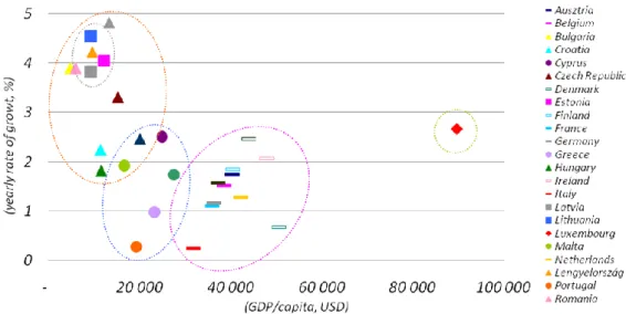
As the first step we conducted a cluster analysis, in which we wanted to see which groups of counties followed the same growth pattern throughout the 10 years of our study. We conducted the analysis in two dimensions: on the one hand, we examined the actual level of economic development in the given national economies based on the yearly GDP data; on the other hand, we studied the pace of growth based on the growth data. For visualization, Figure 1 represents the procedure, where the 10-year averages can be found, depicting growth patterns in two dimensions.

(5)

~ 97 ~

Figure 1. Growth clusters in the European Union

To eliminate divergences rising from the extent of variables before conducting the cluster analyze we standardized the values, which in the practice means that they were divided by the respective deviations. As a result, we can identify five different groups -as shown in Figure 1-, where it is statistically proven that they followed the same growth path.

A striking emergence is the value of Luxemburg, where high economic development is accompanied by a strong medium pace of growth (Cluster 2). The Baltic countries belong to the 1^st group of the analyzing software: Latvia, Lithuania and Estonia are characterized by a high pace of growth and a rather low level of economic development; therefore, they form a separate growth cluster by themselves. Countries in the way of transition, which –due to their historical background- are lagging behind the traditional EU member states form Cluster 3 (Czech Republic, Hungary, Poland, Romania, Croatia, Slovenia, Slovakia and Bulgaria). Their market economies were underdeveloped; however their pace of growth was medium or high throughout the last ten years.

The Mediterranean countries form the 4^th group of the cluster analysis (Spain, Portugal, Malta, Cyprus, and Greece). They were not forced into the socialist planned economy, thus, they had a higher initial level of development, however, the pace of growth is slower here than in the Central and East European countries. The 5^th and last group is formed by the traditional national economies of the Union (11 elements), which –from among the EU15- were able to improve their developed market economy by a pace of growth over 1%.

As the final result of the analysis we can differentiate between the growth patterns of 5 groups of countries, which will be referred to hereafter under the following collective names:

- Cluster 1: the “Baltic states” (Latvia, Lithuania, Estonia);

- Cluster 2: Luxemburg;

- Cluster 3: “CEE countries” (Czech Republic, Hungary, Poland, Romania, Croatia, Slovenia, Slovakia, Bulgaria);

- Cluster 4: the “Mediterraneans” (Spain, Portugal, Malta, Cyprus, Greece);

- Cluster 5: “EU11” (Germany, France, Denmark, the Netherlands, Belgium, Sweden, Finland, Italy, Ireland, Austria, Great-Britain).

(6)

~ 98 ~

The appropriateness of the analysis’ fitting is shown by the distance between the single elements and the cluster center (Annex 1), which –e.g. in case of Italy- both visually and numerically shows an intermediate position located between the Mediterraneans and the EU11 group.

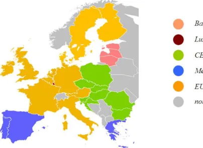
At the end of step one, we can state that the cluster groups formed by the statistical analysis and the growth groups of real economic relationships coincide, their geographic configuration is shown in the following figure 2.

Figure 2. Location of clusters

In the second round of the analysis we intended to discover where were those time periods throughout the examined 10 years in which a European growth model can be exactly identified and described by a function. To identify the patterns we used principal component analysis, which examines which years can be substituted by a common principal component in the further analyses.

The Kaiser-Meyer-Olkin index – which is the measure for sampling adequacy- is 0.802 (Annex 2), which value is meritorious. The communality values, indicating the percentage of the original variables’ information content still present after the principal component analysis, are also presented in the above Annex.

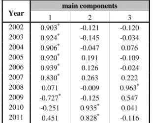
The results of the principal component analysis are shown in Table 1, which –referring to the examined 10 years- indicates which principal component the aggregated growth data of the national economies fit the most. By running the program it can be clearly seen that the period of conjuncture between 2002 and 2007 can be identified with one component (Principal Component 1), and then 2008 was an extreme year of negative growth, which forms a group by itself (Principal Component 3). The year 2009 got into the 1^st group in the analysis, however, as it can be seen in the Table, with a minus sign, which reveals an opposite direction to the 6-year trend. The time period following the economic crisis (2010, 2011) forms Group 2, representing a separate Principal Component. This – reflecting the real growth data – means a new growth pattern.

For the adequacy of the analysis stands on the one hand the high value of the KMO index, on the other hand all those growth periods have been organized in one principal component that can be traced in the practice as well.

(7)

~ 99 ~

Table 1. Results of the principal component analysis Year

main components

1 2 3

2002 0.903^* -0.121 -0.120 2003 0.924^* -0.145 -0.034 2004 0.906^* -0.047 0.076 2005 0.920^* 0.191 -0.109 2006 0.939^* 0.126 -0.024

2007 0.830^* 0.263 0.222

2008 0.071 -0.009 0.963^* 2009 -0.727^* -0.125 0.547 2010 -0.251 0.935^* 0.041 2011 0.451 0.828^* -0.116 Note: * indicates the principal component in that year

3.2 Growth Regression

The previous two subsections presented how the unified economic patterns of the European Union can be decomposed to country groups by cluster analysis, then, we turned our attention to the time scale and studied similar growth periods by running a principal component analysis. In the third and last part of this paper we are going to study whether the created three principal components and the individual growth data are able to interpret the nominal economic output and facilitate predictions.

As result variable- as the first step of regression calculation- we define the GDP of 2011 that we wanted to interpret using the above 3 principal components. The value of R^{2 -} which can be found in Annex 3- is slightly higher than 0.3, indicating the rather low descriptive power of the model. Although beta coefficients can be identified in the regression, thus the mathematical equation can be also formulated, the change of the variables was necessary because of the low descriptive power.

In the second attempt, in order to reach a more adequate result, instead of the value of the nominal GDP in 2011 we used the pace of growth as result variable. Annex 4 presents that the descriptive power of the reformulated regression model is above 90%, however, we need to consider among the boundaries of the analysis that the growth value of 2011 –besides the result variable- is placed in the 2^nd principal component of the explaining variable as well.

In the third round the until now used reduced number of explaining variables got exempted and those original 10 variables (pace of growth in 10 years) were inserted in the model, which explain the economic output of 2011 on nominal value. Annex 5 presents that R²in this case is about 0.6, which descriptive power is considered to be sufficient. The Annex presents the beta values of 10 variables and the constant coefficient, which – in mathematical form- describes the GDP values of the year 2011 on the base of the growth data of the preceding years as follows:

 R₁ = β₀+ β₁*f₁ + β₂*f₂ + … + β_n*f_n

 GDP2011 = 37.497 + 3.109*grw2002 – 6.404*grw2003 + 6.844*grw2004 –

722*grw₂₀₀₅ – 6.113*grw₂₀₀₆ + 5.244*grw₂₀₀₇ – 5.090*grw₂₀₀₈ + 1.505*grw₂₀₀₉ + 2.161*grw2010 - 958*grw2011

(8)

~ 100 ~

4. Concluding Summary

As the purpose of this paper, we defined the presentation of divergences in growth patterns and the synthetisation of single development periods on an econometric basis, in which exact correlations can be shown. The main virtue of the analysis is that the groups of countries with the same economic backgrounds, moving on the same track in real life form separate economic clusters in our model, which can be presented on the map and delineated in space.

The 3 growth periods presented in empirical Part coincide as well with the growth trends of the European economy, and the principal component analysis identifies unambiguously the new growth path after the economic crisis. From among the analysis the results of the regression can be hardly interpreted in economic terms, this, however, might serve as step one in a future research intending to identify economic growth of the different years using other macroeconomic input parameters.

References

[1] Bradley, S.-Taylor, J. (1996). "Human capital formation and local economic performance", Regional Studies, 30(1): 1-14.

[2] Brugges, E.A. (1981). "Innovation-oriented Regionalpolitik: Notizen zu einer neuen Stategia", Geographische Zeitschrift, 68: 173-198.

[3] Lengyel I.-Rechnitzer J. (2004). Regionális gazdaságtan. Dialóg Campus Kiadó, Budapest–

Pécs (In Hungarese).

[4] Lukesch, R. (1981). "Selbsorganisation und autonomie Regionalentwicklung", Österreische Zeitschrift für Politikwissenschaft, 10: 319-332.

[5] Nikodémus A.-Ruttkay É. (1994). A gazdasági modernizáció elemei a hazai regionális fejlődésben. Budapest. Kandidátusi értekezés.

[6] Rechnitzer J. (1990). "Szempontok az innováció térbeli terjedésének kutatásához", In: Tóth J.

(szerk.) Tér-Idő-Társadalom. MTA RKK, Pécs. pp.48-62.

[7] Richardson, H.W. (1973). Regional Growth Theory. London: MacMillan.

[8] Sala-i-Martin, X. (1996a). "The classical approach to convergence analysis", The Economic Journal, 106(437): 1091-1036.

[9] Sala-i-Martin, X. (1996b). "Regional cohesion: evidence and theories of regional growth and convergence", European Economic Review, 40(6): 1325-1352.

[10] Solow, R.M. (1973a). "On Equlibrium Models of Urban Location", In: Parkin, M.-Nobay, A.R.

(Eds.) Essays in Modern Ecominics, London: Logmans, pp.3-16.

[11] Solow, R.M. (1973b). "Congestion Cost and the Use of land for Streets", The Bell Journal of Econimics and Management Science, 4(2): 602-618.

[12] Stöhr, W.B. (1986). Regional Innovation Complexes. Reginal Sciences Papers, vol.59, no.1 [Online] Awailable at http://onlinelibrary.wiley.com/doi/10.1111/j.1435-5597.1986.tb00980.x/

abstract.

[13] Stöhr, W.B. (1987). "A területfejlesztési stratégiák változó külső feltételei és új koncepciói", Tér és Társadalom, 1.sz. pp.96-113(In Hungarese).

[14] Thoss, R. (1983). "Qulitives Wachstum in den Raumordnungsregionen der Bundesrepublik Deutschland", Veröffentlichungder Akademiae für Raumforschung und Landesplanung, nr.104. pp.1-23. (In Hungarese).

(9)

~ 101 ~

Annexes

Annex 1. Clusters and the member distance from the cluster centers cluster distance from the cluster center

Austria 5 0.7999

Belgium 5 0.94016

Bulgaria 3 1.72883

Croatia 3 2.04862

Cyprus 4 1.5981

Czech Republic 3 1.56704

Denmark 5 2.0782

Estonia 1 1.69112

Finland 5 1.55158

France 5 1.2284

Germany 5 1.9498

Greece 4 3.83125

Hungary 3 2.87616

Ireland 5 3.74606

Italy 5 2.16195

Latvia 1 1.93768

Lithuania 1 2.10721

Luxembourg 2 0

Malta 4 2.8334

Netherlands 5 1.32112

Lengyelország 3 2.7059

Portugal 4 2.20519

Romania 3 2.7308

Slovakia 3 2.64199

Slovenia 3 2.07572

Spain 4 1.33289

Swenen 5 2.40658

Great Britain 5 1.45082

Note: The cluster analysis is made of standardized data.

Annex 2. Results of Principal Component Analysis KMO and Bartlett's Test

Kaiser-Meyer-Olkin Measure

of Sampling Adequacy 0.802

Approx. Chi-Square 249.287 Bartlett's Test of Sphericity d.f. 45

Sig. 0.000

(10)

~ 102 ~

Communalities Initial Extraction grw02 1.000 .844 grw03 1.000 .876 grw04 1.000 .828 grw05 1.000 .895 grw06 1.000 .898 grw07 1.000 .808 grw08 1.000 .933 grw09 1.000 .843 grw10 1.000 .939 grw11 1.000 .902

Extraction Method: Principal Component Analysis Communality values of Principal Component Analysis

EU States Factors

F1 F2 F3

Austria -0.68192 0.37037 0.05556

Belgium -0.87315 0.22752 0.02311

Bulgaria 0.97035 -0.43164 1.4606

Croatia 0.4487 -1.26711 0.04453

Cyprus -0.24287 -0.25788 1.01212

Czech Republic 0.34655 0.3866 0.70493

Denmark -0.98006 -0.02806 -0.83702

Estonia 1.64889 1.43061 -1.93515

Finland -0.25719 0.72236 -0.43141

France -0.98846 0.02999 -0.373

Germany -1.19532 1.10605 -0.18328

Greece 0.1083 -3.50985 -0.1662

Hungary -0.11207 -0.4818 -0.62516

Ireland 0.443 -0.88701 -1.23303

Italy -1.25288 -0.09874 -0.9185

Latvia 2.38533 0.17979 -2.00508

Lithuania 2.04948 0.42939 0.03144

Luxembourg 0.04599 0.40957 -0.2178

Malta -0.86992 0.5585 0.74653

Netherlands -0.90216 0.09097 0.21349

Lengyelország 0.03475 1.11082 1.94027

Portugal -1.36593 -0.53168 -0.32987

Romania 1.2022 -0.94061 1.8292

Slovakia 1.01164 1.13723 1.73257

Slovenia 0.32703 -0.30798 0.57201

Spain -0.27097 -0.79031 -0.08839

Swenen -0.50259 1.57744 -0.47628

Great Britain -0.52671 -0.23454 -0.54619

(11)

~ 103 ~

Annex 3. Results of regression

(Independent variables: main components; Dependent variable: GDP 2011) Coefficients

Independent Variables

Unstandardized Coefficients

Standardized

Coefficients t Sig.

B Std. Error Beta

(Constant) 33291.071 3714.570 8.962 0.000

REGR factor score 1 for analysis 1

-

10050.734 3782.733 -0.450 -2.657 0.014 REGR factor score 2

for analysis 1 3981.989 3782.733 0.178 1.053 0.303

REGR factor score 3

for analysis 1 -6236.806 3782.733 -0.279 -1.649 0.112 Model Summary

R R² Adjusted R² Std. Error of the Estimate

0.559 0.312 0.226 19655.66

Four Predictors: (Constant), REGR factor score 3 for analysis 1;

REGR factor score 2 for analysis 1; REGR factor score 1 for analysis 1.

(Independent variables: main components; Dependent variable: growth 2011) Coefficients

Independent Variables

Standardized

Coefficients Collinearity Statistics

B Std. Error Beta Tolerance VIF

(Constant) 1.806 0.169

REGR factor score 1 for

analysis 1 1.216 0.173 0.451 1.000 1.000

analysis 1 2.232 0.173 0.828 1.000 1.000

analysis 1 -0.313 0.173 -0.116 1.000 1.000

Model Summary

R R² Adjusted R² Std. Error of the Estimate

0.950 0.902 0.890 0.89644

Four Predictors: (Constant), REGR factor score 3 for analysis 1;

REGR factor score 2 for analysis 1; REGR factor score 1 for analysis 1.

(12)

~ 104 ~

(Independent variables: yearly growth; Dependent variable: GDP 2011) Coefficients

Standardized

Coefficients Collinearity Statistics

B Std. Error Beta Tolerance VIF

(Constant) 37497.416 12608.251

grw02 3109.170 4270.374 0.288 0.151 6.607

grw03 -6404.507 3151.703 -0.783 0.160 6.265

grw04 6844.628 3995.620 0.650 0.164 6.086

grw05 -722.925 4312.240 -0.079 0.106 9.406

grw06 -6113.304 4686.250 -0.692 0.084 11.893

grw07 5244.949 2967.068 0.603 0.204 4.909

grw08 -5090.540 1630.299 -0.677 0.503 1.986

grw09 1505.773 1688.324 0.275 0.249 4.010

grw10 2161.530 3200.278 0.212 0.240 4.159

grw11 -958.557 2862.770 -0.116 0.198 5.041

Model Summary

R R² Adjusted R²

Std. Error of the Estimate 0.773 0.597 0.360 17868.02973

Eleven Predictors:

(Constant), grw11, grw08, grw03, grw07, grw09, grw10, grw04, grw02, grw05, grw06