M E T H O D O L O G Y A R T I C L E Open Access
Evaluation of whole exome sequencing as an alternative to BeadChip and whole
genome sequencing in human population genetic analysis
Zoltán Maróti1*†, Zsolt Boldogkői2†, Dóra Tombácz2,3, Michael Snyder3and Tibor Kalmár1*
Abstract
Background:Understanding the underlying genetic structure of human populations is of fundamental interest to both biological and social sciences. Advances in high-throughput genotyping technology have markedly improved our understanding of global patterns of human genetic variation. The most widely used methods for collecting variant information at the DNA-level include whole genome sequencing, which remains costly, and the more economical solution of array-based techniques, as these are capable of simultaneously genotyping a pre-selected set of variable DNA sites in the human genome. The largest publicly accessible set of human genomic sequence data available today originates from exome sequencing that comprises around 1.2% of the whole genome (approximately 30 million base pairs).
Results:To unbiasedly compare the effect of SNP selection strategies in population genetic analysis we subsampled the variants of the same highly curated 1 K Genome dataset to mimic genome, exome sequencing and array data in order to eliminate the effect of different chemistry and error profiles of these different
approaches. Next we compared the application of the exome dataset to the array-based dataset and to the gold standard whole genome dataset using the same population genetic analysis methods.
Conclusions:Our results draw attention to some of the inherent problems that arise from using pre-selected SNP sets for population genetic analysis. Additionally, we demonstrate that exome sequencing provides a better alternative to the array-based methods for population genetic analysis. In this study, we propose a strategy for unbiased variant collection from exome data and offer a bioinformatics protocol for proper data processing.
Keywords:WGS, WES, BeadChip, Population genetics, PCA, Admixture
Background
The investigation of the ethnogenesis of human populations is made possible by population genetic studies, through com- paring genetic makeup and frequencies of the selected vari- ants or alleles, and also by computing their genetic distance from the rest of the studied population or their level of ad- mixture [1,2]. Compared to their more costly whole genome sequencing (WGS) counterparts, these assays predominantly
use array-based genotyping techniques (various Human BeadChip arrays /610, 640, 650, 1 M/, Infinium Multi-Ethnic BeadChip arrays from Illumina, Affymetrix Genome-Wide Human SNP Array, Affymetrix Human Origin Array, etc.) that include single nucleotide polymorphism (SNP) sets based on the evaluation of previous genome sequencing data (CEPH, HGP, HapMap databases), with the emphasis on population-specific, ancestry-informative markers (AIMs).
AIMs were first introduced in 2008 by Halder and colleagues [3], as a panel of 176 autosomal AIMs that were capable of effectively distinguishing individual biogeographical ancestry and admixture proportions from among four continental ancestral populations. The importance of
* Correspondence:maroti.zoltan@med.u-szeged.hu;sztegdl.pedia@med.u- szeged.hu;kalmar.tibor@med.u-szeged.hu
†Zoltán Maróti and Zsolt Boldogkői contributed equally to this work.
1Department of Pediatrics and Pediatric Health Center, Faculty of Medicine, University of Szeged, Szeged, Hungary
Full list of author information is available at the end of the article
© The Author(s). 2018Open AccessThis article is distributed under the terms of the Creative Commons Attribution 4.0 International License (http://creativecommons.org/licenses/by/4.0/), which permits unrestricted use, distribution, and reproduction in any medium, provided you give appropriate credit to the original author(s) and the source, provide a link to the Creative Commons license, and indicate if changes were made. The Creative Commons Public Domain Dedication waiver (http://creativecommons.org/publicdomain/zero/1.0/) applies to the data made available in this article, unless otherwise stated.
AIMs has palpable significance in the medical field as well. While case-control design studies can be an effi- cacious strategy for identifying candidate genes in complex diseases in a population, in diversely admixed populations (e.g. Latin Americans, with ad- mixture of American Indians, Europeans and Afri- cans) population stratification can affect association studies and thereby could lead to false genetic associ- ations [4]. This undesirable distortion can be mini- mized by genotyping AIMs.
Ultimately, application of the Whole Exome Sequen- cing (WES) method had spread and gained popularity, as WES is cost effective for routine genetic diagnosis of rare inherited diseases, and extensive databases have been generated containing thousands of publicly access- ible exomes (Exome Aggregation Consortium ~ 61000 exomes [5], Exome Variant Server ~ 6500 exomes [6]). A typical WES dataset contains 100,000 to 130,000 variants (if all the high coverage reads are also analyzed, includ- ing the flanking regions of exons). In rare disease diag- nostics, focus is on filtering out all non-disease specific variants and to find the one or two causative mutations that lead to the disease phenotype. In practice, all rare and common variants aid the exploration of disease vari- ants only as population controls. Since exome data by definition contains high portion of the functional vari- ants that are under selection pressure, in this study, we explored whether this could lead to any bias in popula- tion genetic analysis.
Thus, we assessed the usability of exome data in com- parison with the other approaches in population genetic analyses. In order to compare the practicality of each strategy – (the genome data as unbiased standard, the commonly used array data, and the potentially usable exome data) – we generated three subsets of the same publicly available experimental data (HGP ~ 2,500 unre- lated genomes), accordingly (GENOME, EXOME and BEADCHIP datasets). The results we obtained from these datasets were compared using the most widely used population genetic calculations (including Fixation index (FST), Principal Components Analysis (PCA), f3−
and f4−statistics, admixture) by utilizing the commonly used tools: EIGENSOFT [7], ADMIXTOOLS [8], Admixture [9] and TreeMix [10].
Migration, admixture, adaptation, and genetic drift lead to genetic diversity between human populations. By studying genetic diversity within and between popula- tions, we could reconstruct how these populations are related to one another. Fixation index a measure of gen- etic structure developed by Sewall Wright [11, 12] can be estimated fromgenetic polymorphismdata. FSTis the proportion of the total genetic variance contained in a subpopulation (S) relative to the total genetic variance (T). Its values can range from 0 to 1, where FST= 0
implies panmixia (absence of any differentiation among subpopulations) and FST= 1 implies complete divergence between populations.
Principal Components Analysis is the most widely used approach for identifying ancestry differences among a group of individuals [13, 14]. When applied to genotype data, it calculates principal components (or eigenvectors), which can be viewed as continuous axes of variation that reflect genetic variation due to ancestry in the sample. In- dividuals with similar values for a particular top principal component will have similar ancestry for that axes.
Application of principal components to genetic data from European samples [13] showed that among Europeans for whom all four grandparents originated in the same coun- try, the first two principal components computed using 200,000 SNPs could geographically map their country of origin quite accurately.
F-statistics measure shared genetic drift among sets of populations and can be used to test simple and complex hypotheses about admixture events between populations [15]. Thef3-statistics is used for testing the relationship of three populations [16] by allowing the detection of the presence of admixture in a population C from two other populations, A and B. If the value F3(C; A, B) is negative, then C does not appear to form a simple tree with A and B, but instead appears to be a mixture of A and B. If F3is zero, it indicates the absence of admixture, while a positive F3value implies simple tree-like relations among A, B and C (however, it does not reject admixture). Because of the complex genetic ancestry of human populations, there usually exists more than one possible model for any stud- ied case. The f4-statistics has been developed in order to test alternative hypothetical trees [17]. The f4-statistics is used to estimate the admixture proportion of a test popu- lation (PC) under the assumption that we have a correct historical model. In this test,PA andPB are the potential contributors andPI is a reference population with no dir- ect contribution toPC.
Admixture analysis is based on the maximum likelihood estimation of individual ancestries from multi-locus SNP genotype datasets [9, 18]. It estimates the best possible sources and proportions of admixing components for any hypothetical number (K) of admixing sources. Visualization of admixture components offers an insight into the genetic structure of the studied populations.
Because there is no publicly available WGS data from modern Hungarians and since our results indicate that the use of exome data is suitable for population genetic analysis, we carried out population genetic analysis of modern Hungarians based on their exome data (HUN EXOME dataset). Based on our results, we also evalu- ated a strategy to filter exome data and offer the most suitable parameters for using them in population genetic analysis.
Results
The BEADCHIP dataset contained markedly higher amount of linked markers
Some population genetic approaches like PCA or ad- mixture analysis are based on the assumption of link- age equilibrium. Thus, it is important that linked markers are pruned from the datasets as linkage dis- equilibrium (LD) between tightly linked markers causes certain haplotypes to be more frequent than expected and large blocks of markers in complete LD can seriously distort the eigenvector/eigenvalue struc- ture [7]. This is especially important in the exome dataset as exons of genes, or genes could be tightly packed in small, transcriptionally active chromosome regions. Therefore, we altered the recommended 50 kb sliding window [9] in the –indep-pairwise algorithm of Plink to 10,000 kb, while maintaining the recommended 10 SNPs increment and r2 thresh- old of 0.1. The variant counts and the effect of LD pruning on the different datasets are summarized in Additional file 1: Table S1.
Interestingly, the BEADCHIP dataset, even with the 50 kb sliding window, contained a much higher propor- tion of linked markers (~ 86%) compared to the GEN- OME (~ 52%) and EXOME (~ 55%) datasets. As expected, the larger pruning window affected mostly the EXOME dataset (~ 19% additional markers pruned), while the GENOME (~ 11%) and BEADCHIP (~ 9%) datasets were affected to a lesser degree.
FSTvalues based on the BEADCHIP dataset are
systematically overestimated between populations with larger genetic distance
For each dataset, we calculated the pairwise FST value between each studied population and compared the re- sults of the different datasets (Additional file 2: Table S3). In general, the FST distances generated from the GENOME and EXOME datasets were found to be nearly identical. However in the EXOME dataset we found very small but systematic differences between the FSTvalues of African (except in the LWK African population) and European populations and the African and East Asian populations. We observed that FSTvalues calculated on the basis of the BEADCHIP dataset were systematically overestimated between populations originating from dif- ferent super-populations.
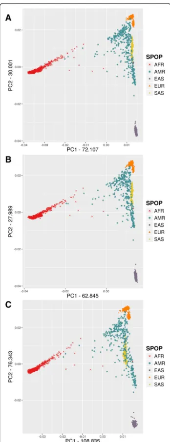
Eigenvalues are notably larger for the BEADCHIP dataset compared to GENOME and EXOME datasets in PCA For each dataset, we performed the PCA analysis of all samples without outlier removal. The different datasets show a remarkably similar overall picture by the first two eigenvectors (Fig. 1a-c). The relative po- sitions of the super-populations are almost the same,
and we can even pinpoint several outlier individuals – for example, some individuals with African ances- try, marked by red dots in the middle – that are po- sitioned in a very similar pattern in each dataset. The greatest difference is that the absolute values of ei- genvectors are significantly larger for the BEADCHIP dataset compared to the GENOME and EXOME data- sets, while the EXOME dataset has the most similar eigenvector values to the GENOME dataset. The complete logs of all PCA analyses on the different datasets (containing detailed Tracy-Widom statistics, average divergence between populations, ANOVA sta- tistics for population differences along each eigen- vector, statistical significance of differences between populations and list of eigen best SNPs) are summa- rized in Additional file 1: DATA/PCA. According to the detailed statistics included in the logs the three datasets showed similar statistical power to differenti- ate populations.
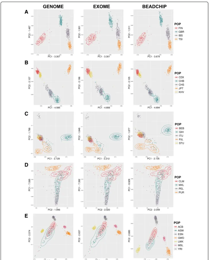
In order to investigate whether the BEADCHIP and EXOME datasets represent similar population relations within each super-population in comparison to the GENOME dataset, next we performed the PCA analysis restricted to each super-population using default outlier removal (removing individuals with > 6 SD of topk ei- genvectors). The detailed PCA of the populations for each super-population showed that the indicated eigen- vectors and values were very similar in all three datasets (Fig. 2a-e). The greatest difference between the three datasets was seen in the AFR super-population. The dif- ferences between the overlap of the historically known admixed ASW and ACB African populations and their relations to the other African populations indicated slightly different population affiliations in the BEAD- CHIP dataset compared to the GENOME and EXOME datasets.
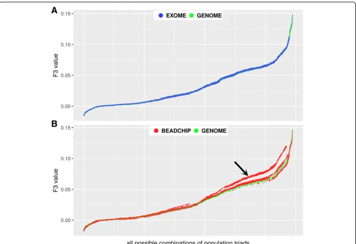
f3-statistics of BEADCHIP dataset deviates from GENOME dataset
In order to compare the usability of the three datasets we calculated the f3-statistics for all possible combina- tions of population triads and plotted the resulting F3
values Fig.3.
Figure 3a shows that the EXOME F3values is almost identical to GENOME results (Pearson correlation r= 0.9998), while the BEADCHIP data (Fig. 3b) presents less correlation (r= 0.9911) with the F3values calculated from the GENOME dataset. The differences are con- fined to the larger positive F3 values in our analyzed populations (shown as deviating red dots from green dots in Fig. 3b). The most deviating cases were those where F3 value were calculated between any two East Asian populations in relation to an arbitrary African population.
F4(TSI, X; CHB; YRI) values were comparable in all analyzed datasets
In the analyzed populations, all possible combinations of any four populations result in an exceedingly large in number. In most cases, the relations between these popu- lation combinations would be meaningless. Therefore, in order to test potential bias between the different datasets, we only calculated the f4-statistic corresponding to a well-known East Eurasian-like ancestry of Northern Euro- pean populations [19]. The F4(TSI, X; CHB; YRI) values where X denotes all possible test populations were calcu- lated for each dataset (Additional file1: Figure S1 A-C).
In all analyzed populations, the f4-statistics showed nearly identical East Asian and African components for each dataset. A population with negative values indicates East Asian gene flow, while positive values indicate dom- inant African genetic components in the test population.
The order of populations was the same for all datasets and the relative ratios between the F4values of different populations was nearly identical. The absolute values were significantly higher in the BEADCHIP dataset com- pared to the GENOME dataset, while the EXOME data- set was more similar to it.
Admixture analysis reveals subtle differences between the different datasets
We performed the admixture analysis and calculated the Cross Validation (CV) error for different models (K = 3 to 10) for each dataset. Since the absolute CV error values were significantly higher in the BEADCHIP data- set compared to the GENOME and EXOME datasets, we displayed the relative CV values compared to the lowest fitting model (K = 3) that resulted the highest CV error for each dataset (Additional file1: Figure S2).
The best fitting model of admixture indicated by the minimum of cross validation error was K = 6 in the GENOME, EXOME and HUN-EXOME datasets, how- ever the CV error of the BEADCHIP dataset indicated the K = 9 model as the best fitting model of admixture.
The curve of the CV errors of the BEADCHIP dataset shows that this dataset resulted in very similar alterna- tive models (ranging from K = 7 to 10) with almost iden- tical CV errors. Since the analysis of the different dataset suggested different best fitting admixture models, we vi- sualized both models (K = 6 and K = 9) for each dataset.
The analysis of the best fitting admixture model (K = 6) suggested by both the GENOME and EXOME datasets produced very similar admixture results (Additional file1:
Figure S3). Each color represents a different admixture component (K). The major topology and admixture com- ponents were very similar in each dataset for all analyzed populations however, the BEADCHIP systematically over- estimated the minor admix components compared to the other two datasets (for example, South Asian component
Fig. 1PCA analysis of super-populations using different datasetsa) GENOMEb) EXOMEc) BEADCHIP
Fig. 2Detailed PCA of super-populations:a) European,b) East Asian,c) South Asian,d) Admixed American,e) African
/marked as orange/ in Italian (TSI) or British (GBR) popu- lations denoted by arrows in Additional file1: Figure S3).
The analysis of the best fitting admixture model (K = 9) suggested by the BEADCHIP dataset produced very simi- lar admixture results for each datasets (Additional file1:
Figure S4). The major topology and admixture compo- nents were very similar for each dataset. The major differ- ences compared to the K = 6 model were that in each dataset, the European super-population was split into two and the African super-population was split into three admixing components. The EXOME dataset was again most similar to the GENOME dataset, and again, the ad- mixture of the BEADCHIP dataset systematically overesti- mated the minor admix components compared to the other two datasets (some examples are highlighted by ar- rows in Additional file1: Figure S4).
Overrepresentation of AIMs in the BEADCHIP dataset Our previous population genetic analyses suggested that the variant composition of the BEADCHIP dataset is dif- ferent from the GENOME and EXOME datasets. To test this hypothesis we calculated the variance of minor allele
frequencies (MAF) of the analyzed populations for each SNP and visualized it as a density plot (Fig.4).
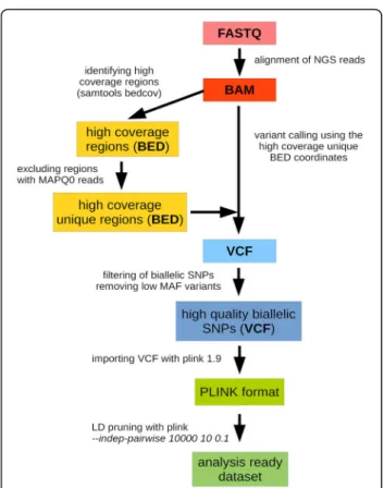
Figure4 shows that SNPs that are highly variable be- tween the test populations are overrepresented in the BEADCHIP dataset, while the distribution observed in the EXOME dataset is nearly identical to the distribution observed in the GENOME dataset. Thus, our analysis also confirms that EXOME dataset does not suffer from the same bias as the BEADCHIP dataset given correct processing of raw sequencing data for which we provide a step-by-step recommendation in Fig.5.
Analysis of the HUN-EXOME dataset
The PCA of the HUN-EXOME dataset (Additional file1:
Figure S5A) shows that Hungarians (denoted by purple circles) belong to the European super-population and that Hungarians are not in close relationship with the other European populations available in the public HGP dataset (Additional file1: Figure S5B).
In the case of Hungarians the F4 (TSI,HUN;CHB;YRI) value (Additional file1: Figure S6) showed that Hungarians have higher East Asian genetic components than the
Fig. 3Comparison of F3 values obtained from the GENOME, EXOME and BEADCHIP datasets. F3 values were ordered and plotted relative to all possible combinations of population triads.a) F3 values from the EXOME vs. the GENOME datasetb) F3 values from the BEADCHIP vs. the GENOME dataset. The arrow denotes substantial deviations from the GENOME F3 values
British population (GBR), but these genetic compo- nents are significantly smaller than those in the Finnish population (FIN).
Since the analysis of the EXOME dataset was compar- able to the other datasets, we also performed the admix- ture analysis of the HUN-EXOME dataset for both the K = 6 and K = 9 models.
In the K = 6 model Hungarians were again classified into the European super-population as the major
admixture component (depicted as blue) is the same as observed in other European populations (Additional file1:
Figure S7A). Within the Hungarian population we can observe a few individuals with significant South Asian genetic components (denoted by orange). In the dataset of analyzed populations considering the K = 9 admixture model (Additional file1: Figure S7B), Europeans display a North-South gradient by the indicated two European specific admix components (represented by the Finnish and Italian populations). According to their geolocation Hungarians are situated in the middle of this gradient having approximately 50–50% portion of these admix components.
Discussion
The WGS, the WES, and the array-based datasets are the three main types of human genetic datasets avail- able today. In this study, we compared the use of these SNP-selection strategies for population genetic analysis, as each method differs in terms of the ratio in which it contains variants under natural selection. Our GEN- OME dataset mainly contains non-exonic variants, since more than 98% of the human genome consists of non-exonic region and our coordinate-based selection was random. The EXOME dataset contains both non-exonic (~ 50%) and exonic variants (~ 50%), al- though only a portion of the exonic variants are func- tional. In order to make the various approaches comparable, we used the same curated HGP 1 kG gen- omic variant data to select the subsets of the GENOME, EXOME and BEADCHIP datasets (see in detail in the Methods section). The number of variants was comparable in all unpruned datasets (Additional file1: Table S1).
Proper LD pruning is a crucial step prior to PCA ana- lysis, as large blocks of completely linked markers may
Fig. 4Density plot of the variation of the minor allele frequencies (MAF) of SNPs between the analyzed populations in the different datasets
Fig. 5Preparation of WES data for population genetic analysis
introduce bias that could result additional eigenvectors [7]. Furthermore, it is also important in admixture ana- lysis, because the calculations assume linkage equilib- rium among the markers [9]. We observed that the unpruned BEADCHIP dataset contained slightly more variants than the GENOME dataset (567 k vs. 483 k variants), but most of them were tightly linked, as only
~ 72 k markers (~ 12%) remained after LD pruning, while in the GENOME dataset the ratio was ~ 43% (~ 205 k markers) which indicates a smaller fraction of linkage. We suppose that these differences are contributed to the tightly linked pre-selected AIMs in the BEADCHIP data- set. The coordinate-based EXOME dataset had somewhat higher linkage than the dispersed GENOME dataset. This is assumed to be a consequence of the organization of the human genome, where genes and exons are not homoge- neously dispersed, but rather tend to be packed tightly in functionally active euchromatic chromosome regions.
Correspondingly, after LD pruning about 149 k, a slightly lower proportion of variants (~ 38%) remained in the EX- OME dataset out of the ~ 405 k unpruned variants. Com- paring the PCA results of the EXOME dataset with the gold standard GENOME dataset, we refined the LD pruning parameters of exome data. We suggest extending the prun- ing window (to 10,000 kb)–while keeping the original 0.1 squared correlation threshold–in order to counter the ef- fect of the packed exome variant composition and to elimin- ate the tightly linked markers. According to our results, this modification did not significantly alter the variants of the BEADCHIP dataset; however, it did eliminate additional tightly linked variants in the EXOME and to a lesser degree in the GENOME datasets Additional file1: Table S1.
The fixation index is one of the most commonly used statistics in population genetics, which is a measure of population differentiation due to genetic structure. The FSTdistances between African (except the LWK popula- tion) and the European populations were very slightly (0.001–0.002) but systematically smaller using the EXOME dataset. On the other hand, the FSTvalues be- tween the African and East Asian populations were very slightly (0.001–0.002) but systematically larger compared to the GENOME FSTdistances. Since this slight difference was systematic between the random GENOME and the EXOME dataset (which by definition contains functional variants besides the non-coding and other functionally inert variants), we hypothesize that a portion of functional variants are accountable for this phenomenon. However, the deviation (~ 1–3%) is still only a portion of what was observed in the BEADCHIP dataset. The comparison of FSTvalues of the BEADCHIP dataset to the GENOME dataset revealed that the pairwise FST distances between populations of different super-populations were systemat- ically larger (~ 1–12%), and that the extent of the differ- ence appears to be correlated to the phylogenetic distance.
On the contrary, we detected almost no differences be- tween the FST distances of populations within the same super-population, except in the highly admixed AMR super-population. We assume that this is due to a general overrepresentation of differentiating SNPs (AIMS) and im- balances in the selection and proportion of the marker com- position in the pre-selected BEADCHIP dataset. This hypothesis is also supported by the observed FSTvalues of the admixed ASW population. The ASW population is a sub-population of African Americans in the Southwestern United States who originated from West-Africa, and later mixed with Caucasian and American Indians. Accordingly, the BEADCHIP data places this population closer to its admix sources - the European (EUR) and Admixed Ameri- can (AMR) super-populations - than those of the GENOME FSTvalues, indicating that the overrepresentation of AIMs distorts the true population distances. As FSTcan be used to estimate coalescence times [20,21], significant deviations in FSTvalues - such as observed using the BEADCHIP dataset - may lead to bias in these estimations.
For each dataset the PCA analysis showed both similar topology and comparable relations between the analyzed populations. We observed that for the first two eigenvec- tors of the whole dataset (Fig.1a-c) the eigenvalues were greater in the BEADCHIP dataset compared to the GENOME dataset, while the EXOME datasets were more similar to it. The eigenvalue with the largest abso- lute value is known as the dominant eigenvalue and can be used to determine the rate of growth in the popula- tion [22]. An overestimation of the eigenvalues miscalcu- lates the population growth rate. The largest differences between the detailed PCA were seen in the African super-population (Fig.2e) where the BEADCHIP dataset gave slightly different eigenvalues and population rela- tions compared to the GENOME and EXOME datasets.
Similarly to the FSTresults, the admixed ASW and ACB populations displayed slightly different relations to other populations. We assume that again, the overrepresenta- tion of AIMs in the BEADCHIP dataset is responsible for the increased eigenvalues and the different relations of the admixed ASW and ACB populations. Nonethe- less, the genetic relationship among the studied popula- tions was still comparable.
Comparison of the three datasets showed that the GENOME and the EXOME data gave almost identical F3 values (r= 0.9998 Fig. 3a), while the Z scores were slightly smaller in the EXOME dataset, which was attrib- utable to the smaller SNP count. On the other hand, the f3-statistics of the BEADCHIP dataset showed less cor- relation (r= 0.9911 Fig.3b). The Z scores of thef3-statis- tics in the BEADCHIP dataset were also higher, even though the SNP count was about one third of the GEN- OME dataset, which indicates higher deviation from the mean. Plotting the corresponding F3 values revealed
systematic differences in a large portion of population combinations between the BEADCHIP and GENOME datasets. Investigation of F3values showed that tree like split of East Asian populations from African populations was systematically overestimated by the f3-statistics based on the BEADCHIP dataset. We assume that this bias is due to the overrepresentation of AIMs between the East Asian and African populations within the pre-selected variants of the BEADCHIP dataset. Taking all this together, we conclude that the EXOME data is highly suitable for f3-statistics. Although the absolute F3
value deviation from zero is meaningless if we only test whether f-statistics is consistent with zero [8] (meaning no admixture), the inferred magnitude of relatedness in comparison to relations between other populations may lead to bias or overinterpretation of data in some spe- cific cases (such as where markers are not evenly repre- sented in the analyzed populations) of the BEADCHIP dataset (due to higher F3values and optimistic Z score- s).On the other hand our analysis supports thatf4-statis- tics is robust to SNP ascertainment (all three datasets resulted in nearly identical proportions) and deviation from zero is only observed if the test population is admixed [8].
The admixture analysis of different datasets suggest different best-fit admix modelsSince the BEADCHIP dataset resulted in higher CV errors and a number of very similar alternative models, it appears that this dataset is less conclusive for pinpointing the true ad- mixture model. Nevertheless, the admixture analysis of the different datasets resulted very similar admixture components for all of the tested models (Additional file1:
Figures S3-S4). The observed overrepresentation of minor admixture components in the BEADCHIP dataset may lead to overestimation of their admix ratios.
In our comparative analyses, we used the same HGP dataset to make an unbiased assessment of the different strategies of variant selection. However, comparing data- sets from different sources may lead to bias due to the differences in the applied NGS variant calling tools, pipelines, thresholds, and quality of sequences. The ma- jority of genotyping uncertainties stem primarily from the fact that various NGS pipelines use slightly different (only partially overlapping) quality parameters and pipe- line specific fix tresholds which is not always optimal for analyzing all genomic regions with different read depths (due to inter-sample and/or target region variances)..
Thus, in order to minimize the bias, we applied a num- ber of criteria for exome data processing before using them for population genetic analyses. Hence, we ex- cluded the low-coverage data, based on the real coverage profile of our aligned NGS reads, as these data may have led to ambiguous variant calls. We excluded all read length variations (INS/DELS/DUPS) from the analysis
since the same variant may be represented ambiguously by different variant callers. We also excluded potentially pseudogenic, conservative and repetitive regions where reads could be ambigiously mapped to multiple genomic regions and the proportion of the alternatively aligned sequencing reads may lead to differences depending on the threshold values or the pipeline applied for the analysis.
Using these strict criteria, we merged the Hungarian ex- ome data and analyzed the resulting HUN-EXOME dataset with the appropriate population genetic tools.
Both the PCA and admixture analysis of the modern Hungarian exome dataset confirms that genetically, modern Hungarians are Europeans (Additional file 1:
Figure S5 PCA; Additional file 1: Figure S7 K = 6, K = 9 admixture plots). We note here that our admixture ana- lysis (K = 9) indicated two genetic components with a North-South European gradient which has a ~ 50–50%
portion in Hungarians. Admixture analysis also detected a portion of a South Asian component in a few individuals of the Hungarian population, which in our view can be attrib- uted to the Gypsies living as an ethnic minority (~ 5%) in Hungary. F3analysis of HUN-EXOME dataset also suggests a small but significant (high Z scores) South-Asian-HUN admixture (Additional file1: Table S2).
Historically, gypsy tribes left India in the 9th and 10th centuries as a result of Muslim attacks in areas they inhabited and first appeared in territory of the medieval Kingdom of Hungary in the 14th and 15th centuries, probably fleeing from the conquering Turks in the Bal- kans [23]. This assumption is also supported by the fact that the South-Asian genetic component is confined to only a few Hungarian individuals with high contribu- tions indicating a recent admixture. Unfortunately we cannot explicitly verify the ethnic origin as our exome data was anonymous and therefore we had no informa- tion on ethnicity. Modern Hungarians identify them- selves as having originated from the Hungarian Conquerors, who are deemed to have arrived to the Carpathian Basin in the ninth Century migrating from around the Ural Mountains, which is the natural border between Europe and Asia. The f4-statistic indicated a small East Asian admixture component in modern Hun- garians (Additional file 1: Figure S6) that was also seen as minor admixture components in few Hungarian indi- viduals (Additional file 1: Figure S7). The minor East Asian component detected in modern Hungarians is possibly the genetic trace of Hungarian Conquerors as also suggested by mtDNA analysis [24, 25]. Because the publicly available HGP dataset contains worldwide pop- ulations with no or very little genetic relation to modern Hungarians, our analysis indicated only known and plausible relations of modern Hungarians in relation to the analyzed populations (such as general European
ancestry with small-scale East-Asian components and a recent admixture with South-Asian components). How- ever, this systematic analysis confirms the usability of WES data in population genetic analysis and leads us to conclude that exome data from populations having shared ethnogenesis with Hungarians could result in an even bet- ter understanding of their genetic history.
Conclusion
Overall, our comparative analysis indicates that the array-based preselected SNP-set (BEADCHIP dataset) deviates most from the GENOME dataset. The reason behind this phenomenon may be twofold. First, the pre-selection of SNPs in the array is not necessarily a uniform representation of all of the analyzed popula- tions, and second, the increased proportion of AIMs is shifting the balance towards highlighting the differences between populations. The increased proportion of AIMs makes the BEADCHIP dataset suitable for sensitive ex- ploration of admixture components. However, it could also lead to deviations of the Fixation index, specific cases of f3-statistics, PCA eigenvalues, suggested admix- ture model, and admixture rates. Thus, all derived pa- rameters (e.g. coalescent time, population growth rate) estimated from these statistics are prone to bias in case of array-based data. WES data, on the other hand, is not affected by this bias and is suitable for population gen- etic analyses. Based on the usability of the EXOME data- set we would encourage everyone to use and to publicly share WES sequences with the correct indication of eth- nic and geographical origin, which could contribute to- wards a better understanding of the genetic relationships among human populations.
Methods
Preparation of Hungarian exome data
Our previously published BAM files of Hungarian whole exomes [26] were aligned by the BWA-MEM algorithm [27]. Using the whole cohort, we identified the high coverage regions (all samples in the cohort had coverage
>10x) using samtools bedcov (version 1.3.1) algorithm [28] with the SureSelect V5 all exon plus UTR kit mani- fest bed coordinates. Since some of the regions may con- tain repetitive elements or pseudogenic regions with non-unique sequences, we excluded all regions that had anyMAPQ0reads (mapping quality 0, indicating that the read could be mapped to multiple genomic regions). We excluded sex chromosomes from the analyzed regions. As a result, we generated a BED coordinate list (Additional file 1: Data/HighCov_HighQual_EXOME.bed) that con- tained the high coverage, unique genomic regions of the exome kit. Variant calling was performed by the GATK HaplotypeCaller(version 3.5) best practice [29] using the parameters-stand_emit_conf 10 -stand_call_conf 30in the
HaplotypeCaller module, and --ts_filter_level 99.0 in the variant recalibration (ApplyRecalibration) module. We fil- tered the variants to include only high quality SNPs (PASS filter) in the final high coverage/unique bed regions. We also filtered out multi-allelic variants and variants that had
< −0.5 InbreedingCoeff (indicating variants that violate HW equilibrium, which would potentially be technical er- rors since our cohort consisted of unrelated patients).
Preparation of public datasets
We used the publicly available variants from the higly cur- rated VCF files of the Human Genome Project 1 kG phase 3 dataset [30]. We excluded the geographically inaccurate CEU population and all of the related individuals from our analysis. Our final dataset included sequence data of 2,369 individuals originating from 25 available populations, as follows: European (EUR: GBR - British in England and Scotland; FIN - Finnish in Finland; IBS - Iberian popula- tions in Spain; TSI - Toscani in Italy), South Asian (SAS:
BEB - Bengali in Bangladesh; GIH - Gujarati Indian in Houston TX; ITU - Indian Telugu in the UK; PJL - Punjabi in Lahore, Pakistan; STU - Sri Lankan Tamil in the UK), East Asian (EAS: CDX - Chinese Dai in Xishuangbanna, China; CHB - Han Chinese in Bejing, China; JPT - Japanese in Tokyo, Japan, KHV - Kinh in Ho Chi Minh City, Vietnam; CHS - Southern Han Chinese, China), Admixed Americans (AMR: CLM - Colombian in Medellin, Colombia; MXL - Mexican Ancestry in Los Angeles, California; PEL - Peruvian in Lima, Peru; PUR - Puerto Rican in Puerto Rico), and African (AFR: ASW - African Ancestry in Southwest US; ACB - African Caribbean in Barbados; ESN - Esan in Nigeria; GWD - Gambian in Western Division, The Gambia; LWK - Luhya in Webuye, Kenya; MSL - Mende in Sierra Leone; YRI - Yoruba in Ibadan, Nigeria).
To compare the capabilities of the sequencing-based (WES and WGS) and array-based approaches, we cre- ated three SNP datasets (denoted as EXOME, GENOME and BEADCHIP) established upon the following rules:
first, the EXOME dataset (Additional file 1: Data/EX- OME) was prepared by filtering the public 1 kG variants with the bedtools intersect algorithm using the genomic coordinates of the high-coverage high-quality exome BED coordinate list that we established using the Hungarian exome data. Second, the GENOME dataset was created on the basis of a homogeneously dispersed genomic coordinate list that spanned all somatic chro- mosomes (Additional file 1: Data/GENOME.bed). The first and last 5 Mb of the telomeric regions of chromo- somes were excluded in order to eliminate uncertain se- quences, such as repetitive elements. The remaining genomic regions on each chromosome was equally di- vided; the first 258 base pairs in every 10 kb DNA stretch were used by thebedtools intersectalgorithm for
extracting homogeneously dispersed variants across the genome (Additional file1: Data/GENOME). The resulting unbiased genomic region coordinates were found to have a cumulative size (68.7 Mb), which is similar to the cumu- lative size of the high-coverage exome regions (68.9 Mb).
In order to prepare the BEADCHIP dataset (Additional file1: Data/BEADCHIP), the genome coordinates of a fre- quently used Human genotyping array kit (Illumina Human610-Quad BeadChip) were used from the kit’s manifest file and converted to BED coordinates. Thebed- tools intersectalgorithm was used to filter the correspond- ing variants from the 1 kG genomic variants. From all three datasets, we removed all multi allelic variants, along with variants that were found in less than 10 individuals (or in all but 10 individuals in case of refseq error). This resulted in comparable variant numbers for each dataset (567 k BEADCHIP, 405 k EXOME, 483 k GENOME). The 1 kG annotated joint VCF was re-coded toplink.pedand plink.mapformats. Plink (version 1.9) was used to gener- ate the binary bed format files used in the downstream analysis [31].
Merging Hungarian exome data with public dataset In order to create the merged HUN-EXOME dataset, we used the same high-coverage high-quality exome BED co- ordinate list, which we established using Hungarian ex- ome data, and thebedtools intersectalgorithm for filtering the variants in both the Hungarian exome data and the 1 kG datasets. The filtered exome and 1 kG variants were merged with the GATK CombineVariants algorithm. We removed multi allelic variants, as well as variants that were only found in less than 10 individuals (or all but 10 indi- viduals in case of refseq error). The resulting joint VCF were re-coded toplink.pedandplink.mapformats and we used plink to generate the binary bed format file (Add- itional file1: Data/HUN-EXOME).
LD pruning of datasets
LD pruning was carried out using the –indep-pairwise algorithm of plink (version 1.9). Because of the structure of the human genome, it was expected that exome vari- ants would yield non-homogeneously dispersed markers.
Therefore, we performed the LD pruning using different sliding window sizes (the recommended 50 kb of admix- ture protocol, and an extended 10,000 kb) to prune linked markers in order to identify the best parameters.
For both window sizes, we kept the recommended 10 SNPs increment and r2threshold of 0.1 to allow pruning of markers by the same linkage criteria. In order to allow unbiased comparison of the three methods, we used the same LD pruning parameters (10,000 kb sliding window, 0 SNPs increment and r2 threshold of 0.1) for each dataset.
FSTand PCA calculations
The pairwise FSTmatrix and the PCA analysis of popula- tions were performed by the EIGENSOFT software (ver- sion 6.1.3) [7] on the LD pruned datasets. For each subset of data (whole dataset and the different super-populations), the LD pruning of linked variants and the subsequent PCA calculations were performed separately. PCA analysis was carried out without outlier removal for the whole datasets and with outlier removal (SmartPCA config file, outliersigma tresh SD = 6) for the analysis of individual populations for each super-popula- tion. PCA plots were visualized by ggplot2 (version 2.2.1) [32].
f3and f4-statistics
The F3tests were carried out by theqp3Popprogram of ADMIXTOOLS [8] for each population triad of the ana- lyzed populations. The F4tests were calculated using the fourpop algorithm of TreeMix software (version 1.13).
For each dataset, the corresponding F4(TSI,X;CHB,YRI) values were calculated (where X refers to the given test population). F3and F4values of the tests were visualized by ggplot2.
Admixture analysis
Admixture analysis was performed by the ADMIXTURE software (version 1.3.0) using the LD pruned datasets with the--cvoption for K = 3 to 11 values using 20 itera- tions and randomized seeds [9]. The best admixtures suggested by the cross-validation plots of genome/ex- ome and BEADCHIP datasets were visualized by a cus- tom Perl script using Linux ImageMagick software (version 6.7.7–10).
Additional files
Additional file 1:Table S1.Number of high-quality biallelic variants in GENOME, EXOME, BEADCHIP, and HUN-EXOM datasets before and after LD pruning.Table S2.f3-statistics of Hungarian and selected South Asian populations indicate admixture which could be attributed to the Gypsies living as an ethnic minority in Hungary.Figure S1.The f4 (TSI, X; CHB;
YRI) statistics estimates the East Asian and African components for each dataset. Negative values indicates East Asian gene flow, while positive values indicate dominant African genetic components.Figure S2.Calcu- lated CV error for different admixture models (K=3 to 10). The best fitting model of admixture indicated was K=6 in the GENOME, EXOME and HUN-EXOME datasets, however, it was K=9 in case of the BEADCHIP data- set.Figure S3.Admixture analysis of 25 populations with the K=6 admix- ture model. The major topology and admixture components were very similar in each dataset for all analyzed populations but the minor admix components were systematically overestimated using the BEADCHIP dataset.Figure S4.Admixture analysis of 25 populations with the K=9 admixture model. Besides the minor admix components overestimation using BEADCHIP this admixture model suggested that the European super-population was split into two and the African super-population was split into three admixing components.Figure S5.PCA of the HUN- EXOME dataset confirms that genetically, modern Hungarians belong to the European super-population and within the Europeans, two genetic components exist with a North-South European gradient.Figure S6.
F4(TSI, X; CHB, YRI) values of the HUN-EXOME dataset indicates that Hun- garians have higher East Asian admixture component than British but lower than Finnish population.Figure S7.Admixture analysis of 25 popu- lations using the HUN-EXOME dataset for the A) K=6 and B) K=9 admix- ture models. Besides the major Europian admixture component in few Hungarian individuals minor East Asian admixture components also de- tected. Data Supplementary Data was deposited to:https://figshare.com/
s/e91794c7141a7eb16255. (PDF 2255 kb)
Additional file 2:Table S3.The calculated FST and FST difference data used for analyses. FST matrix of populations based on the GENOME, EXOM, BEADCHIP datasets.The difference between the FST matrix of the GENOME and EXOME, GENOME and BEADCHIP datasets. FST matrix of populations based on the HUN-EXOME dataset. (XLSX 34 kb)
Abbreviations
ACB:African Caribbean in Barbados; AFR: African; AIMs: ancestry-informative markers; AMR: Admixed American; ASW: African Ancestry in Southwest US;
BEB: Bengali in Bangladesh; CDX: Chinese Dai in Xishuangbanna, China;
CEU: Utah residents with Northern and Western European ancestry; CHB: Han Chinese in Bejing, China; CHS: Southern Han Chinese, China; CLM: Colombian in Medellin, Colombia; CV: Cross Validation; EAS: East Asian; ESN: Esan in Nigeria; EUR: European; FIN: Finnish in Finland; FST: Fixation index;
GATK: Genom Analysis Toolkit; GBR: British in England and Scotland;
GIH: Gujarati Indian in Houston,TX; GWD: Gambian in Western Division, The Gambia; IBS: Iberian populations in Spain; ITU: Indian Telugu in the UK;
JPT: Japanese in Tokyo, Japan; KHV: Kinh in Ho Chi Minh City, Vietnam;
LD: linkage disequilibrium; LWK: Luhya in Webuye, Kenya; MSL: Mende in Sierra Leone; MXL: Mexican Ancestry in Los Angeles, California; PCA: Principal Components Analysis; PEL: Peruvian in Lima, Peru; PJL: Punjabi in
Lahore,Pakistan; PUR: Puerto Rican in Puerto Rico; SAS: South Asian; STU: Sri Lankan Tamil in the UK; TSI: Toscani in Italy; WES: Whole exome sequencing;
WGS: Whole genome sequencing; YRI: Yoruba in Ibadan, Nigeria
Acknowledgements Not Applicable.
Funding
No funding was received.
Availability of data and materials
The higly currated VCF files of the Human Genome Project 1 kG phase 3 dataset was avaiable atftp://ftp.1000genomes.ebi.ac.uk/vol1/ftp/release/
20130502/. BAM files of Hungarian whole exomes are previously published (Scientific reports2017,7(1):7106.) and was deposited at the Sequence Read Archive (SRA) under BioProject SUB2335490). All data generated or analyzed during this study are included in this published article and in Additional file 1: Data deposited to figshare (https://figshare.com/s/
e91794c7141a7eb16255).
Authors’contributions
All authors contributed to conceiving the project and analysis design, ZM did the formal analysis. DT, ZB, TK and ZM evaluated the results of the analyses. ZM and TK wrote the initial version of the manuscript while ZB, DT and MS contributed to subsequent versions. All authors reviewed and approved the final version of the manuscript.
Ethics approval and consent to participate Not applicable.
Consent for publication Not applicable.
Competing interests
The authors declare that they have no competing interests.
Publisher’s Note
Springer Nature remains neutral with regard to jurisdictional claims in published maps and institutional affiliations.
Author details
1Department of Pediatrics and Pediatric Health Center, Faculty of Medicine, University of Szeged, Szeged, Hungary.2Department of Medical Biology, University of Szeged, Faculty of Medicine, Szeged, Hungary.3Department of Genetics, School of Medicine, Stanford University, Stanford, CA, USA.
Received: 20 April 2018 Accepted: 15 October 2018
References
1. Hellenthal G, Busby GBJ, Band G, Wilson JF, Capelli C, Falush D, Myers S. A genetic atlas of human admixture history. Science. 2014;343(6172):747–51.
2. Li JZ, Absher DM, Tang H, Southwick AM, Casto AM, Ramachandran S, Cann HM, Barsh GS, Feldman M, Cavalli-Sforza LL, et al. Worldwide human relationships inferred from genome-wide patterns of variation. Science.
2008;319(5866):1100–4.
3. Halder I, Shriver M, Thomas M, Fernandez JR, Frudakis T. A panel of ancestry informative markers for estimating individual biogeographical ancestry and admixture from four continents: utility and applications. Hum Mutat. 2008;
29(5):648–58.
4. Stefflova K, Dulik MC, Barnholtz-Sloan JS, Pai AA, Walker AH, Rebbeck TR.
Dissecting the within-Africa ancestry of populations of African descent in the Americas. PLoS One. 2011;6(1):e14495.
5. Lek M, Karczewski KJ, Minikel EV, Samocha KE, Banks E, Fennell T, O'Donnell- Luria AH, Ware JS, Hill AJ, Cummings BB, et al. Analysis of protein-coding genetic variation in 60,706 humans. Nature. 2016;536(7616):285–91.
6. NHLBI GO Exome Sequencing Project (ESP), Seattle, WA (02/2018) [http://
evs.gs.washington.edu/EVS/]. Accessed Feb 2018.
7. Patterson N, Price AL, Reich D. Population structure and eigenanalysis. PLoS Genet. 2006;2(12):e190.
8. Patterson N, Moorjani P, Luo Y, Mallick S, Rohland N, Zhan Y, Genschoreck T, Webster T, Reich D. Ancient admixture in human history. Genetics. 2012;
192(3):1065–93.
9. Alexander DH, Novembre J, Lange K. Fast model-based estimation of ancestry in unrelated individuals. Genome Res. 2009;19(9):1655–64.
10. Pickrell JK, Pritchard JK. Inference of population splits and mixtures from genome-wide allele frequency data. PLoS Genet. 2012;8(11):e1002967.
11. Slatkin M. Inbreeding coefficients and coalescence times. Genet Res. 1991;
58(2):167–75.
12. Wright S. The genetical structure of populations. Ann Eugenics. 1951;
15(4):323–54.
13. Novembre J, Stephens M. Interpreting principal component analyses of spatial population genetic variation. Nat Genet. 2008;40(5):646–9.
14. Price AL, Patterson NJ, Plenge RM, Weinblatt ME, Shadick NA, Reich D.
Principal components analysis corrects for stratification in genome-wide association studies. Nat Genet. 2006;38(8):904–9.
15. Peter BM. Admixture, population structure, and F-statistics. Genetics. 2016;
202(4):1485–501.
16. Reich D, Thangaraj K, Patterson N, Price AL, Singh L. Reconstructing Indian population history. Nature. 2009;461(7263):489–94.
17. Keinan A, Mullikin JC, Patterson N, Reich D. Measurement of the human allele frequency spectrum demonstrates greater genetic drift in east Asians than in Europeans. Nat Genet. 2007;39(10):1251–5.
18. Pritchard JK, Stephens M, Donnelly P. Inference of population structure using multilocus genotype data. Genetics. 2000;155(2):945–59.
19. Reich D, Patterson N, Campbell D, Tandon A, Mazieres S, Ray N, Parra MV, Rojas W, Duque C, Mesa N, et al. Reconstructing native American population history. Nature. 2012;488(7411):370–4.
20. Hudson RR, Slatkin M, Maddison WP. Estimation of levels of gene flow from DNA sequence data. Genetics. 1992;132(2):583–9.
21. Weir BS, Cockerham CC. Estimating F-statistics for the analysis of population structure. Evolution. 1984;38(6):1358–70.
22. Caswell H. Matrix population models: construction, analysis, and interpretation. 2nd ed: Sinauer Associates Inc; 2000. ISBN-10: 0878930965, ISBN-13: 978-0878930968.
23. Kemeny I. History of Roma in Hungary. In: Roma of Hungary. Boulder:
Publisher Social Science Monographs. p. 1–69.
24. Biro A, Feher T, Barany G, Pamjav H. Testing central and inner Asian admixture among contemporary Hungarians. Forensic science international Genetics. 2015;15:121–6.
25. Tomory G, Csanyi B, Bogacsi-Szabo E, Kalmar T, Czibula A, Csosz A, Priskin K, Mende B, Lango P, Downes CS, et al. Comparison of maternal lineage and biogeographic analyses of ancient and modern Hungarian populations. Am J Phys Anthropol. 2007;134(3):354–68.
26. Tombacz D, Maroti Z, Kalmar T, Csabai Z, Balazs Z, Takahashi S, Palkovits M, Snyder M, Boldogkoi Z. High-coverage whole-exome sequencing identifies candidate genes for suicide in victims with major depressive disorder. Sci Rep. 2017;7(1):7106.
27. Li H: Aligning sequence reads, clone sequences and assembly contigs with BWA-MEM.https://arxiv.org/abs/1303.3997; 2013.
28. Li H, Handsaker B, Wysoker A, Fennell T, Ruan J, Homer N, Marth G, Abecasis G, Durbin R. Genome project data processing S: the sequence alignment/
map format and SAMtools. Bioinformatics. 2009;25(16):2078–9.
29. Van der Auwera GA, Carneiro MO, Hartl C, Poplin R, Del Angel G, Levy- Moonshine A, Jordan T, Shakir K, Roazen D, Thibault J, et al. From FastQ data to high confidence variant calls: the Genome Analysis Toolkit best practices pipeline. Current Protocols Bioinformatics. 2013;43(11.10):11–33.
30. Genomes Project C, Auton A, Brooks LD, Durbin RM, Garrison EP, Kang HM, Korbel JO, Marchini JL, McCarthy S, McVean GA, et al. A global reference for human genetic variation. Nature. 2015;526(7571):68–74.
31. Chang CC, Chow CC, Tellier LC, Vattikuti S, Purcell SM, Lee JJ. Second- generation PLINK: rising to the challenge of larger and richer datasets.
GigaScience. 2015;4:7.
32. Wickham H: ggplot2: Elegant Graphics for Data Analysis: Springer-Verlag New York; 2009.https://doi.org/10.1007/978-0-387-98141-3.