IMPLEMENTING THE INTELLIGENT DRIVER MODEL IN A PHYSICAL VEHICLE SIMULATOR
Tamás Kovács 1*
1 Department of Information Technology, GAMF Faculty of Engineering and Computer Science, John von Neumann University, Hungary
https://doi.org/10.47833/2021.3.CSC.001
Keywords:
vehicle-simulator Intelligent Driver Model Article history:
Received 30 Oct 2021 Revised 15 Nov 2021 Accepted 22 Nov 2021
Abstract
The Intelligent Driver Model was introduced in 2000 by M. Treiber et al. as a mathematical car following model for traffic micro- simulation. It is an obvious question whether this model is applicable in physical vehicle simulator, which would be a big step forward a real application. Of course, it is also essential that the model can be applied to the description of real traffic conditions - thus also to take into account the real speed-density relationship [10]. In the present work this model is implemented in the CARLA physical vehicle simulator. First the simulators acceleration-control functions are established. These functions give the amount of throttle or brake control values to achieve the desired acceleration. Having these functions the Intelligent Driver Model is implemented and tested with simple simulation experiments.
1 Introduction
The computer simulators used for examining road-traffic scenarios can be divided into three main groups depending on the mathematical tools and simulated details. The mathematically most abstract group is formed by the so called macro-simulators. In these the road (or lane) network is treated as a directed graph, and the traffic flow is modeled as a current on the links with different resistances. The next step toward a more detailed model is the group of micro-simulators where the movement of each individual vehicle, that is the speed-time functions and the lane-changes, are described by a mathematical formula. Since the main purpose of these formula is to keep an optimal following speed and distance to the leader car, they are often called as car-following models. The Intelligent Drive Model (IDM) [1], [2], introduced by Treiber et al. in 2000, become a popular such a formula for micro-simulators due to its simplicity and stabile behavior. In Section 2 it will be introduced in details.
The third and most detailed group of the simulators is formed by the physical vehicle simulators. Here the movements of the vehicles are calculated by a mechanics simulator engine considering the relevant technical and physical parameters of the vehicle (such as engine power, maximal torque, wheel’s friction, etc.). That is, the vehicle is controlled by not simply a speed-time function of some mathematical model, but by simulated throttle, steering wheel and brake. Here I omit the detailed introduction of all of the known physical simulators. Instead, only the CARLA simulator, which applied in the present work, will be introduced in the Section 3.
In Section 4 the simulation experiments and the results are introduced and in the last section a short conclusion is given.
* Corresponding author. Tel.: +36 76 516 412 ; fax: -
2 Car-following algorithms
The question arises that whether it is possible to implement a mathematically given car- following model (of a micro-simulator) with a physical simulator. Considering an autonomous (or, with other words, self-driving) car, such a car-following algorithm is essential, and in the past decade numerous control algorithms are published to solve this problem. Best et al. [3], for example, divide the vehicle trajectory into smaller segments and try to find the optimal control values for each of the segments by an optimization solver. They work with a hybrid objective function that includes a term rewarding fast proceeding towards the destination, a term punishing unsafe following distances or speeds and a term ensuring convenient (tolerable) acceleration values. Once the desirable speed value and direction vector are given, a PID controller is applied to achieve the desired speed and turning angles.
Zhao et al. [4] use a somewhat similar mathematical model to the IDM to get the desired following speed and distance. The next is an optimization stage to treat the time-lag of the controls and other disturbances and finally they also use PID control for setting the throttle, brake and steering.
In the Intelligent Driver Model (IDM) [1], [2], the vehicle's behavior is defined by a parameter set, and the input are given by the kinematics variables, i.e. the relative position and the speed of the leader vehicle. In this model only the desired longitudinal (parallel to the speed) acceleration of a vehicle is given by the equations below, where v is the speed of the vehicle, Δv is the speed- difference between the ego and the leader vehicles, s is the distance between the two vehicles and s* is the ideal following distance.
𝑎𝑙𝑜𝑛 = 𝑎0[1 − (𝑣
𝑣0)𝛿− (𝑠∗(𝑣,∆𝑣)
𝑠 )2] (1)
where
𝑠∗(𝑣, ∆𝑣) = 𝑠0+ 𝑚𝑎𝑥 [0, (𝑣𝑇 + 𝑣∆𝑣
2√𝑎0𝑏)
2
] (2)
This model can be considered to be a control system, where the velocity is the controlled parameter, and the controlling function (alon) depends on the velocity, which is the proportional term (P), and the relative distance, which is the integral term (I). So the system is somewhat similar to the PID control, though the differential term (D) is missing and the other two term is not linear. In order to have a complete control system based on the equations (1) and (2), we need the relationships:
𝑡ℎ𝑟𝑜𝑡𝑡𝑙𝑒 = 𝐹𝑡ℎ(𝑎𝑙𝑜𝑛 , 𝑣) (3)
𝑏𝑟𝑎𝑘𝑒 = 𝐹𝑏𝑟(𝑎𝑙𝑜𝑛 , 𝑣) (4)
that gives the throttle and brake control values as functions (Fth and Fbr) of the desired acceleration.
The determination of these functions in case of the CARLA simulator is detailed in Section 4. It is important to note that the classic IDM model is known to be a collision-free model. Therefore, in critical cases, unrealistic, extreme deceleration values may occur when using the classical model.
and can be used freely. The simulation platform supports flexible specification of sensor suites, environmental conditions, full control of all static and dynamic actors, maps generation. The simulator is working as a server and based on the Unreal Engine 4 game development platform.
This simulator-server can be manipulated from the client side with the help of a Python API. A detailed introduction on the capabilities of CARLA can be read in [5]. Recently, various application areas of the simulator were presented in [6, 7, 8], which indicates the scientific value of this system.
4 Simulation experiments and results
As it was treated in Section 2, first we need to establish the relationship between the desired acceleration of the simulated vehicle and the main engine controls (throttle and brake, see eq. (3)).
In order to get these functions, three series of simulation experiments were accomplished. In the first series a chosen vehicle model (Mercedes-Benz Sprinter) was accelerated on a straight level road by fixed relative throttle values in the range [0.0 .. 1.0] until it reached 17 m/s (61.2 Km/h). The throttle was increased in 0.1 steps from experiment to experiment (The 1.0 value corresponds to full throttle).
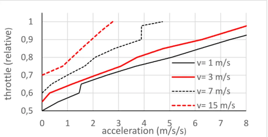
Meanwhile the acceleration phases the speed-time functions were recorded, and hence the acceleration-time functions are obtained by numeric derivation. From these, the function Fth (alon, v) can be derived numerically. The results can be seen on Fig. 1. The function at hand is given only for the case when acceleration (i.e. positive acceleration) is needed. On the figure only a few curves (belonging to a few speed values) are depicted, however, the function Fth (alon, v) was determined for each whole speed values (i.e. for 1 m/s, 2 m/s, 3 m/s, …17 m/s).
Figure 1. The throttle-acceleration curves for four fixed velocities
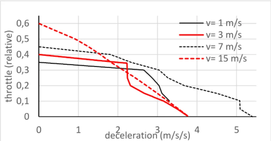
In the next series of experiment the “engine brake region” of the Fth (alon, v) function was established. This is the case when we achieve deceleration by a lower throttle value at a relative high speed, that is, we apply “engine brake” Here the car was accelerated with full throttle on a straight level road until it reached 17 m/s speed, and then a lower throttle value was applied to achieve deceleration (i.e. negative acceleration). With the method given above the negative acceleration region of Fth (alon, v) was obtained. The results are shown in Fig 2.
0,5 0,6 0,7 0,8 0,9 1
0 1 2 3 4 5 6 7 8
throttle (relative)
acceleration (m/s/s)
v= 1 m/s v= 3 m/s v= 7 m/s v= 15 m/s
Figure 2. The throttle-deceleration (engine-brake) curves for four fixed velocities
In the third series of experiment the Fbr (alon, v) function was established (with fixed zero throttle). In this case the car was accelerated also with full throttle until it reached 17 m/s speed, and then a zero throttle value and a non-zero brake value was applied to achieve deceleration. The brake value was in the range [0 .. 1.0] and was increased by 0.1 from experiment to experiment (the 1.0 value corresponds to full brake). The deceleration was established by fitting a linear function on the speed-time data. The results are shown in Figure 3.
Figure 3. The brake-deceleration curve
Having these curves the function-values of Fth (alon, v) Fbr (alon, v) can be obtained by interpolation between the calculated discrete data-points. In the IDM control experiments these functions were used.
In the present work the stopping capability of the IDM control was tested with a simple scenario:
a standing still “leader” car was placed at 160 meters distance and the ego car (Mercedes Sprinter) driven by the IDM accelerated from zero velocity and then decelerated in order to stop behind the standing still leader car. The application of IDM can be summarized as shown in Figure 4. With 50 frames per second update frequency the desired acceleration value was calculated by the IDM based on the momentary distance and speed values. And then, using the above determined Fth (alon, v), Fbr (alon, v) functions the proper throttle and brake values was obtained. If the desired deceleration was greater than the highest possible “engine-brake” deceleration, then a non-zero brake value was applied (given by Fbr (alon, v)), otherwise zero brake value was used, that is, whenever it was possible, engine-brake deceleration was applied. Besides, the algorithm was completed by an emergency brake function, so that full brake (value 1.0) was applied if the ego car approached the leader car
0 0,1 0,2 0,3 0,4 0,5 0,6
0 1 2 3 4 5
throttle (relative)
deceleration (m/s/s)
v= 1 m/s v= 3 m/s v= 7 m/s v= 15 m/s
0 0,2 0,4 0,6
3 5 7 9 11 13
brake (relative)
deceleration (m/s/s)
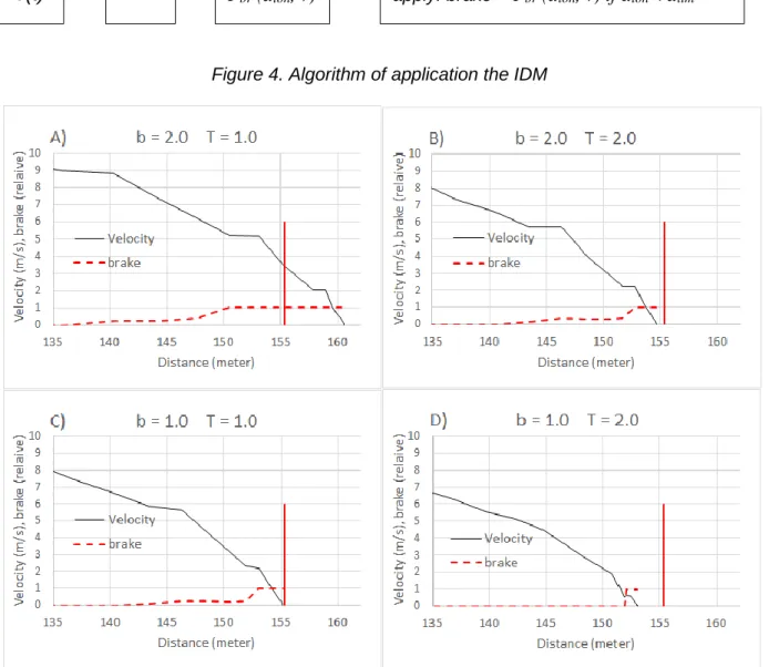
Figure 4. Algorithm of application the IDM
Figure 5. The distance-speed curves and brake values in the stopping experiments controlled by the IDM. The safe stopping point is denoted by a vertical red line on the diagrams. The IDM
parameters b and T are given in m/s/s and sec units in the diagram titles.
Following from the IDM, the ego car should stop at s0=2 (m) (bumper to bumper) distance from the standing still leader. This point is denoted by vertical red lines on the diagrams. It is seen that the ego car was unable to stop in the case of b = 2.0 (m/s/s), T = 1.0 (s) (see diagram A) in spite of the automatic emergency braking function, the velocity decreases to zero well after the desired stop point. The situation is better in the cases of b=2.0 (m/s/s), T=2.0 (s) and b=1.0 (m/s/s), T=1.0 (s): the IDM control is not but the emergency braking function is able to stop the vehicle before reaching the desired stop point. The only ideal case among the four is when the parameters are chosen to be b=1.0 (m/s/s), T=2.0 (s) (see diagram D). The velocity is very small (around 0.5 m/s) when the emergency braking is activated, so it has only a stabilizing function, that is, it prevents the car rolling slowly closer to the leader. In other words, in the case shown by diagram D the IDM control was able to stop the ego vehicle, while in the other three cases it was not.
s(t) v(t)
IDM
Fth (alon, v) Fbr (alon, v)
apply: throttle = Fth (alon, v) if alon> alim
apply: brake = Fbr (alon, v) if alon< alim
5 Conclusion and future possibilities
The original question was that whether it is possible to implement the Intelligent Driver Model in a physical car simulator as a reliable vehicle-following algorithm. The experiments have shown that if the relationship between the desired acceleration and the controls (throttle and brake) can be established, and the parameters of the IDM are chosen carefully, then the implementation of the model is possible i.e. the vehicle following model may be reliable. The term “may be” is used, since no experiments were made related to the cases when the leader is moving. However, the results so far encourage us to make a deeper examination of application the IDM in self-deriving car models in physics simulators, which is a great step towards real applications in test-roads. This can render us a useful tool for investigation of self-driving algorithms with lower-emission rates. It should be emphasized that this research can be extended to other very important research areas. Such a very important field today is research into environmental effects and related emission studies [13], [14], [15].
Acknowledgment
This research is supported by GINOP-2.3.4-15-2016-0001 " Globális jelentőségű járműipari kutatás-fejlesztési központ létrehozása Magyarországon a Bay Zoltán Közhasznú Nonprofit Kft., a Neumann János Egyetem és az AVL Hungary Kft. Együttműködésében " project. The Project is supported by the Hungarian Government and co-financed by the European Social Fund.
References
[1] Treiber, M.,D. Helbing, D.: Congested traffic states in empirical observations and microscopic simulations, Phys.
Rev. E 62, (2000) 1805-1824
[2] Treiber, M., Helbing, D.: Microsimulations of freeway traffic including control measures. Automatisierungstechnik 49, (2001) 478-484
[3] Best, Andrew, et al. "Autonovi: Autonomous vehicle planning with dynamic maneuvers and traffic constraints." 2017 IEEE/RSJ International Conference on Intelligent Robots and Systems (IROS). IEEE, (2017)
[4] Zhao, R. C., et al. "Real-time weighted multi-objective model predictive controller for adaptive cruise control systems." International journal of automotive technology 18.2 (2017) 279-292
[5] Dosovitskiy, A., et al. "CARLA: An open urban driving simulator." Conference on robot learning. PMLR, 2017.
[6] Hofbauer, M., et al. "Telecarla: An open source extension of the carla simulator for teleoperated driving research using off-the-shelf components." 2020 IEEE Intelligent Vehicles Symposium (IV). IEEE, (2020)
[7] Dworak, D., et al. "Performance of LiDAR object detection deep learning architectures based on artificially
generated point cloud data from CARLA simulator." 2019 24th International Conference on Methods and Models in Automation and Robotics (MMAR). IEEE, (2019)
[8] Stević, S., et al. "Development and Validation of ADAS Perception Application in ROS Environment Integrated with CARLA Simulator." 2019 27th Telecommunications Forum (TELFOR). IEEE, (2019)
[9] Kovács, T., Bolla, K., Alvarez Gil, R., Csizmás, E., Fábián, Cs., Kovács, L., Medgyes, K., Osztényi, J., Végh, A., 2016, Parameters of the intelligent driver model in signalized intersections, Technical Gazette, 23, No. 5, 1469-1474., https://doi.org/10.17559/TV-20140702174255
[10] Derbel, O., Péter, T., Mourllion B., & Basset M. (2017), Generalized Velocity–Density Model based on microscopic traffic simulation, Transport, DOI: 10.3846/16484142.2017.1292950 To link to this article:
http://dx.doi.org/10.3846/16484142.2017.1292950 ISSN: 1648-4142 (Print) 1648-3480;
http://www.tandfonline.com/loi/tran20- cikk!
[11] Derbel, O.; Peter, T.; Zebiri, H.; Mourllion, B.; Basset, M. (2012). Modified intelligent driver model, Periodica
[14] Lakatos, I.: Instacioner üzemállapotú motorteljesítmény-mérés görgős járműfékpadon, In: Bikfalvi, MicroCAD 2010:
XXIV. microCad International Scientific Conference: E szekció: Anyagtudomány és -technológia Miskolc, Magyarország , Miskolci Egyetem (2010) pp. 33-38., 6 p.
[15] Lakatos, I.: Gépjárműmotorok szelepvezérlése, Győr, Magyarország, Jaurinum Bt. (1994), 132 p.