Dynamics of Mass Variable System Cvetityanin Lívia, PhD MTA doktori értekezés Szeptember 2012

(1)

Dynamics of Mass Variable System

Cvetityanin Lívia, PhD MTA doktori értekezés

Szeptember 2012

(2)

In this dissertation the dynamics of the body and the system of bodies with time variable mass and time variable moment of inertia are treated. Namely, there are a lot of machines, mechanisms and system in practical use which parts are mass variable or have the variable moments of inertia. Let us mention some of them: centrifuges, sieves for sorting particles, transportation mechanisms, lifting mechanisms, cranes, automatic weight measuring instruments, and rotors used in the textile, cable, paper industry, etc. The aim of modern industry is to increase productivity and to fully automate, resulting in various new challenges in the dynamics of systems and machines with nonlinearities and mass and also moment of inertia variation. The both types of mass and moment of inertia variation are considered: the discontinual and the continual. The basic lows in dynamics are extended to the case when the mass is varying in time. The principle of momentum and of angular momentum are applied to obtain the velocity and angular velocity of the body after discontinual mass variation. The same results are applied analytically by introducing the procedures of analytical mechanics. The dynamics of mass addition is treated as the plastic impact, and of the separation as the inverse process to plastic impact. For the case of the continual variation of the mass and of the moment of inertia in time, beside the reactive force, the reactive torque is introduced. The case of the free motion of the mass variable body is investigated. The Lagrange’s equations of motion are derived. As the special motion of the mass variable body, the vibration is considered. The main attention is given to approximate solving of the strong non-linear differential equations of motion. The influence of the reactive force on the vibration properties of the body is analyzed. This dissertation based on the dynamics of the particle with time variable mass and the basic laws of dynamics, in this dissertation the theoretical consideration of the dynamics of the body and system of bodies with time variable mass and moment of inertia are given. The dissertation is divided into following Chapters:

After the Introduction, various mechanisms and machines with variable mass and moment of inertia are shown. The construction and also the working properties of the machines and mechanisms are described.

In Chapter 2, the linear momentum and the angular momentum of the body with variable mass and moment of inertia are considered. The linear and angular momentum of the body before and after mass modification due to adding or separating of the mass are determined. These values are the fundamental ones for dynamic analysis of the bodies with discontinual or continual time variable properties.

In Chapter 3, the obtained linear and angular momentum relations are applied for calculation of the velocity and angular velocity of the body when the body separation or augmentation is discontinual. The principles of momentum and angular momentum are used as the basic ones. The special case of the in-plane separation is considered. Depending on the type of motion of the separated body, the kinematic properties of the remainder body are discussed. An example the dynamics of a crumbled rotor is discussed according to the fact of separation of a body from the initial one.

In the Chapter 4, the dynamics of the discontinual mass variation is treated by analytically, by using the principles of analytical mechanics. An analytical procedure for the velocity and angular velocity determination of a body in the process of mass variation is developed. The main attention is given to the case when no external forces and torques act. The process of body addition is treated as the plastic impact and the separation as an inverse process of the plastic impact of bodies. An example of separation of a rotating pendulum into two bodies is treated.

In the Chapter 5, we express the free motion of the body with continual time variation of the mass and moment of inertia. Due to mass and also moment of

(5)

inertia variation, beside the reactive force, the reactive torque acts. In this section the main attention is directed toward investigation of the influence of these two physical actions. As a special type of motion the in-plane motion of the body is considered. The obtained theory is applied for analyzing of the plane motion of the rotor on which the band is winding up.

In the Chapter 6, the Lagrange’s equations of the motion for the body with continual variation of mass and moment of inertia is derived. The generalized forces due to the reactive force and the reactive torque are defined. The obtained Lagrange’s equations represent the analytical description of the free motion of the body with variable mass.

The Chapter 7, the vibrations as a special type of the motion of the body with variable mass. Based on the general equations of motion given in the Chapter 6, the mathematical model for the oscillatory motion is formed. The main attention is directed to approximate solution procedures for solving the strong nonlinear differential equations with slow-time variable parameters de- scribing the vibrations of various kinds of oscillators. Various types of oscillators are treated: one-degree-of-freedom oscillators, two-degree-of-freedom one-mass oscillators (rotors) and also the oscillators which contain two masses and have two-degrees-of-freedom. Specially the influence of the reactive force and of the reactive torque on the vibration properties of the system with variable mass and moment of inertia are investigated.

In the dissertation the conclusions and remarks for the future Investigations are given in Chapter 8.

The dissertation ends with the Reference list.

(6)

1 Introduction

The problem of the motion of mass variable systems is evident since the 17th century.

Galileo discovered the anomaly in the Moon motion which he believed is the function of the system mass variation. Lately, Laplace theoretically explained the phenomena of the secular acceleration of the Moon. Dufour, 1886, explained that the mass of the earth varies continuously due to the falling shooting-stars and also due to combustion or spending in the atmosphere. He found that the dust of shooting-stars which fall on the surface of France in one year can cover a volume of0.1m³. Oppalzer, 1884, was the first to analyze the reason for secular acceleration of the Moon as the result of Earth and Moon mass increase. Namely, during a hundred year a2.8mmdust layer is formed on the Earth. Gylden, 1884, extended the previous investigations in celestial mechanics by analyzing of the relative motion of two variable mass systems under influence of the Newton force. Meshchersky, 1893, continued the investigation and found that the body with variable mass would move along a spiral, tending toward zero, or it would increase the distance to the other mass variable system.

Cayley in his works (Cayley, 1857; 1858) was the first to consider the influence of the continual mass variation on the motion of the body. The class of the dynamic problem he studied was the ’continuous reactive problem’, i.e., the problem when continuously the infinitesimal small mass is added to a system which causes the velocity of the system continuously to be changed for a definite value. The two most widely discussed examples were (see Cayley, 1859): one, the chain is on the table and is dropping vertically down from the table, and the second, the chain is moving straightforward on a horizontal plane without friction under the influence of a mass M which is fixed at the end of a chain which is rolling around a drum and changing the length during motion.

At the end of the nineteenth century and at the beginning of the twentieth Meshch- ersky, 1897, laid the foundations of the modern dynamics of a particle with variable mass. After that publication numerous investigations have been done and the dynamics of variable mass systems is developed. In the ’variable mass systems’ particles are expelled and /or captured during motion.

Two kinds of systems are identified:

- ’continuously’ particle-ejecting systems, where the mass variation is a continual function of the time, position (see Grudtsyn, 1972) or velocity of the particle, and

- ’discretely’ particle-ejecting systems, where the mass variation is a discontinual function (for example, automatic weapons that fire rounds, one at a time).

For the case of discontinual mass variation Meshchersky, 1952, calculated velocity of the particle after mass variation. The finite discontinual mass variation in a very short time was not of special interest for a long time and was not intensively discussed.

Meshchersky was the first to consider the velocity change of a translatory moving body during step-like mass variation. Mass which is separated or added has a finite amount and the mass variation of the body is discontinual. The theory is mostly applied for solving of the Keplerian twobody problem (see Luk’yanov, 2005), and also the three and four-body problems (Cveticanin, 2007).

The motion of the continuously mass variable systems is much more investigated due to its application in rocket theory (Meirovitch, 1970; Cormelisse et al, 1979;

Tran & Eke), astronomy (Kayuk & Denisenko, 2004), for charged particle motion in a magnetic field with decreasing mass and charge (Howard, 2007), in robotics (McPhee & Djerassi, 1991; Djerassi, 1998) in machinery (Cveticanin, 1984; 1988; 1989;

1991; 1993₁; 1993₂; 1995; 1998₁; 2001) etc. The motion is described with differential equations with variable parameters (Kayuk & Tivalov, 1987; Wang & Eke, 1995; Eke

& Mao, 2002; Pesce, 2003). The effect of expulsion and /or capture of particles on

(7)

the motion of the continuously mass variable system is evident as changes in the integration variables of the governing dynamic equations. In spite of that the variable mass systems may be conservative (Leubner & Krumm, 1990; Cveticanin, 1994) and with non-holonomic properties (Ge & Cheng, 1982; Ge, 1984). For the case when the mass is continually varying in time, the influence of the reactive force on the motion (see Apykhtin & Jakovlev, 1980; Azizov, 1986; Cveticanin, 1992; 1993₃; 2004) and also on the stability (Ignat’yev, 1991; Cveticanin, 1996₁; 1996₂) were investigated. The reactive force is mathematically the product of the mass variation function and the relative velocity of mass separated or added to the particle. Usually, two special cases were considered: first, the relative velocity is zero and second, the absolute velocity of separated or added mass is zero. If the relative velocity is zero, i.e., the absolute velocity of the separated or added particle is equal to the velocity of the basic particle, then the reactive force is also zero. Levi-Civita, 1928, investigated the motion of the particle for the case when the absolute velocity of the separated or added mass is zero and the reactive force exists. The most comprehensive consideration of the dynamics of the body with variable mass is given in the books of Bessonov, 1967, Conelisseet al.,1979, and Cveticanin, 19982.

In this chapter various types of machines and mechanisms with mass variable elements are described. The expression "variable mass element" or "body with variable mass" as used in the context of this dissertation, refers to mechanical systems that lose and/or gain mass while in motion. Examples of such devices abound in contemporary engineering literature. They include complex systems such as aircraft, rockets, auto- mobiles, moving robots picking up or lifting objects, as well as simpler systems such as transportation machines, mining machines, excavators, vibrating machines used as conveyors, separators, machines for segregation, rolling mills, metallurgical machines, casting machines, agricultural machines, centrifuges, measuring mechanisms, etc. In these mechanisms, the mass of elements and the position of their centre of mass and moment of inertia vary during addition or removal of the material. In this chapter various types of machines and mechanisms with mass variable elements are described.

Their constructive properties and the working procedure are explained.

A pouring machine, shown in Fig.1, represents a mechanism with variable mass.

The hook of the crane grips the vessel at point B, and rotates it around A, pouring out the molten metal for continuous casting. The basic requirement for the equipment is that pouring of metal from the vessel has to be uniform, and it is regulated by the velocity of the hook.

Fig.1. Mechanism for tipping a vessel

(8)

To estimate the process of lifting of the vessel and to give good control it is necessary to take into consideration the mass variation of the vessel, because it is the basic cause of uniform flow of metal. The position of the centre of mass of the vessel and metal varies. As a simplification this system can be considered as a rotating bar AB with variable mass and variable position of the centre of mass inside the element.

Let us consider some other mechanisms. The pouring of concrete from the vessel in Fig.2 is achieved by a mechanism which contains an electric motor 1, which by a system of gears 4 and 6 and screws 2 and 3 transmits the motion to 4. As 4 is fixed to vessel 5 its motion about 6 turns the vessel. To analyze the elements and the process of vessel turning, the variable mass of the vessel has to be taken into account. Only in this way can the correct position of the turning axle and the torque for vessel rotating be obtained.

Fig.2.Mechanism for rotating a vessel

Fig.3. Mechanism for converter turning

Converters are used for steel production. For melting the steel, the converter- vessel system is usually lifted and turned during the introduction some additives and pouring out the finished steel. An electric motor 1 with a system of gear-wheels 2, 3 and 4 rotates the converter 5 (Fig.3). Exact dynamic analysis taking into account

(9)

the variation of the mass of metal in the converter is necessary for automatic control of the process.A system of a rotor type of wagon turner is shown in Fig.4. The wagon with material 1 is in the rotor 2. The rotor rotates on cylinders 3 and is driven with a mechanism 4 and rope 5. The wagon is supported by positioners 6 and 7. By turning the wagon by an angle smaller than 180 degrees discharging is completed.

The efficiency of this mechanism is very high.

Fig.4. Mechanism for wagon turning

The mechanism for discharging wagon which is widely used in the metallurgical industry for minerals is of the rotating type (Fig.5). The wagon 1 is on the carrier 2, and is supported on the wall 3 and elements 4. The rope 5 is turning on the wheel and tips the carrier, discharging the material from the wagon. Torques are balanced with a system of counterweights. The mechanism productivity is high as the discharging is rapid. For dynamic analysis, the mass variation has to be taken into consideration.

Fig.5. Mechanism for discharging a wagon

(10)

Fig.6. Wagon with variable mass

A wagon 2 which moves laterally is shown in Fig.6. It is driven by a motor 1. Another type of laterally moved wagon is shown in Fig.7. Movement in one direction increases the mass and in the other it is decreased. The mechanism is a bar mechanism, and the motion may be reversible. In both mechanisms the mass varies.

A rolling mill is shown in Fig.8. Tin rolls down off the drum 1, travels through the rollers 2 and rolls up on the drum 3. The system is fixed by supporting rollers 4. Cold rolling is caused at a velocity 10 to 15 m/sec and more. During rolling up this tin and rolling it off the radius and the moment of inertia of the drum varies.

One of the most important requirements is constant velocity of rolling up, and special automatic regulation and controls have to be introduced. To increase the efficiency of these machines, the dynamics of motion of this system with variable mass have to be analyzed.

Fig.7. Transportation mechanism

Fig.8. Rolling machine scheme

(11)

Another mechanism with variable moment of inertia is shown in Fig.9.

It is a centrifugal lifting basket regulator of motion. It contains shaft 1, system of gears, and a system of mercury filled tubes. The velocity of the shaft and of the tubes regulates the velocity of the basket. If the velocity of tubes is zero, the level of mercury in all tubes is the same. If the velocity increases, the mercury level attains a parabolic shape and the level in the middle tube decreases. If it gets to a very small level, the connection with the motor is broken and the shaft 1 slows down. If the velocity of basket motion is smaller than permitted, the regulator sets up the motor and transfers the motion to the shaft 1. As the position of the mercury depends on velocity, the moment of inertia varies, as a function of angular velocity, J(w). To give the correct instructions for regulator dynamic behavior it is necessary to know the change of moment of inertia of the mechanism.

Fig.9. Centrifugal regulator

A simple planar model of an excavator is shown in Fig.10. It consists of five rigid bodies: body 1 which is in contact with the ground, body 2 mounted on 1, body 3 connected to 2 by means of pivot, body 4 which is an excavator arm connected with 3 by means of a joint, and body 5 which is the excavator scoop and can rotate around the body 4.

Fig.10. Excavator model

The excavator scoop has a varying mass. The operating movements can be real- ized by means of the jib 3, arm 4 or the scoop 5 movements. A crane represents a mechanism for load transportation.

A typical sectional model of a crane (Fig.11) consists of four rigid bodies: body 1 which is in elastic contact with the ground, body 2 mounted on 1, body 3 connected with 2 by means of joint and a component 4 connected with 3 by a flexible cord.

Component 4 has a time variable mass, because it includes the load. Variation of mass

(12)

and its distribution along the elements of a mechanism have a significant influence on belt type automatic dosing devices.

Fig.11. Sectional model of crane mechanism

The aim of the mechanism is to achieve constant mass flow of material. The mechanism (Fig.12) contains basket 1, belt conveyor 2 and bar mechanism 3. The bar is a sensitive element which directs the opening and shutting of the dosing device.

The process of separating material from the conveyor may result in large vibrations around O. These vibrations are undesirable and they are due to mass variation.

Fig.12. Belt type automatic dosing device

A mechanism for automatic measurement of liquid is shown in Fig.13. It contains bar 1, which is pivoted at 2 and is under the influence of weight 3, and vessel 4 which is to be filled with liquid. The quantity of liquid is regulated by a special dosing device 5 which automatically regulates the liquid in the vessel by stopping the liquid getting in. It is connected to bar 1.

Fig.13. Mechanism for automatic measurement of liquid

(13)

A special group of mechanisms are the rotors with variable mass. Rotors with variable mass are the fundamental working elements of many machines in process, cable, textile and paper industry, as well as in transportation, etc. The term "rotor with variable mass" will refer to all parts which are mounted on the rotating shaft and whose mass is varying. The shaft which is a fundamental element of the rotor is designed to support machine parts rotating with it and to transmit bending moments and torques and also longitudinal forces.

As can be seen, mechanisms with variable mass are widely used in various indus- trial fields: process, transportation, civil engineering, regulators etc. Most of them can be reduced to a simple dynamic model with mass variation which is a function of time (for example, vibration mechanisms, dosing devices, etc). For correct dynamic analysis of the mechanical system it is necessary to take this property of the system into consideration.

(14)

2 Linear and angular momentums for the mass vari- able body

In this Chapter the linear and angular momentums for the bodies in the process of separation or addition of the bodies are determined. These values are necessary to express the general principles of dynamics of system of bodies with variable mass and for mathematical modeling of separation or adding of bodies.

Let us consider the discontinual mass variation caused by the body separation or augmentation. The initial body has the massM and the moment of inertiaI_S with respect to the mass centreS whose position vector due to the fixed pointOisr_S (see Fig.14.).

Fig.14. Position vectors, velocities and angular velocities of the system: a) body separation, b) body augmentation.

The linear velocity of the mass centre isv_S and the angular velocity of the initial body around the mass centreSisΩ.The position vector of the mass centreS to the fixed pointOisrS. The separating or adding body has massmand the mass centre S2. Moment of inertia of that body is I_S2 with respectto the mass centre S2.The absolute velocity of the mass centerS2 isv_S2 while the angular velocity of the body with respect to point of rotationS₂ isΩ₂.The position vector of the mass centreS₂ according to the fixed pointO at the moment of adding or separating isr_S2. If the separation of the body occurs, the remainder body has the mass(M−m)and if the augmentation occurs the mass is(M+m). The moment of inertia of the final body isI_S1due to the mass centreS₁whose position to the fixed pointOis given with the vectorr_S1.The unknown linear and angular velocity of the body after mass variation arev_S1andΩ₁. In the Table 1. the introduced Nomenclature is shown.

The linear momentum of the initial body with massMand velocity of mass center v_S is

K=Mv_S. (1)

If the separated or added massmhas the velocityvS2, its linear momentum is

K₂=mvS2. (2)

After process of separation or addition the final mass isM∓m,where the minus sign is for mass separation and plus sign for mass addition.

(15)

Table 1. Nomenclature.

Initial Final Separated/

body body Added body

Index - 1 2

Mass center S S1 S2

Position of mass center SS₁ SS₂

Position vector of mass center r_S r_S1 r_S2

Mass M M∓m ∓m

Absolute velocity of mass center v_S v_S1 v_S2

Relative velocity of mass center v_r1 v_r

Absolute angular velocity Ω Ω₁ Ω₂

Relative angular velocity Ω_r1 Ω_r

Moment of inertia tensor I_S I_S1 I_S2

Linear momentum K K₁ K₂

Angular momentum relating to O LO LO1 LO2

Angular momentum relating to mass center LS LS1 LS2

Remark 1 In general in this Chapter in any relation, the minus sign is for change of some quantity caused by mass separatiom and the plus sign is for mass addition.

The unknown velocity of the mass centreS1 isvS1 and the corresponding linear momentum is

K₁= (M∓m)vS1. (3) Introducing the assumption that the bodies during the mass separation or addition belong to an unique system (see Fig.14), we obtain the linear momentumsK_b before andK_aafter mass variation:

for mass separation

K_b=K=Mv_S, K_a=K₁+K₂=mv_S2+ (M−m)v_S1, (4) for mass augmentation

K_b=K+K₂=Mv_S+mv_S2, K_a=K₁= (M+m)v_S1, (5) The difference between the linear momentums before and after mass variation is

∆K=M(vS1−v_S)±m(vS2−v_S1). (6) The angular momentum of the initial body before mass variation with respect to the fixed pointO(Fig.14) is

L_O=r_S×Mv_S+L_S. (7) After mass variation the angular of the final body relating to the fixed pointOis

L_O1=r_S1×(M∓m)v_S1+L_S1. (8) The angular momentum of the separated or added body is

LO2=rS2×mvS2+LS2. (9) Dependently on the type of mass variation the angular momentums beforeLOb and afterLOa mass variation are:

(16)

for mass separation

LOb = LO=rS×MvS+LS, (10) L_Oa = L_O1+L_O2=r_S1×(M−m)v_S1+L_S1+r_S2×mv_S2+L_S2, for mass addition

LOb = LO+LO2=rS×MvS+LS+rS2×mvS2+LS2, (11) L_Oa = L_O1=r_S1×(M+m)v_S1+L_S1.

Based on (10) and (11), the difference between the angular momentums is

∆L_O=L_S1±L_S2−L_S+r_S1×(M∓m)v_S1±r_S2×mv_S2−r_S×Mv_S. (12) The relation (6) and (12) are the basic ones for dynamic analysis of the mass variation problems.

For the position of the system mass centerS r_S =M∓m

M r_S1± m

Mr_S2, (13)

and position vectorsr_S1 andr_S2 (Fig.14)

r_S1=r_S+SS₁, r_S2=r_S+SS₂, (14) we obtain

(M∓m)SS₁=∓mSS₂, (15)

Substituting (14) into (12) we obtain

∆LO =LS1±LS2−LS+SS1×(M∓m)vS1±SS2×mvS2. (16) Introducing the relation (6) into (16) it is

∆L_O=L_S1±L_S2−L_S+r_S×∆K∓SS₂×m(v_S1−v_S2). (17) Due to (15) the relation (16) transforms into

∆L_O=L_S1−L_S±L_S2∓SS₂×(v_S1−v_S2)m, (18) i.e.,

∆L_O=I_S1Ω₁−I_SΩ±I_S2Ω₂∓SS₂×(v_S1−v_S2)m, (19) where L_S = I_SΩis the known angular momentum of the initial body before mass variation,LS1=IS1Ω1 depends on the angular velocityΩ1 of the final body with respect toS1and is proportional to the moment of inertiaIS1forS1andLS2=IS2Ω2

is the known angular momentum of the separated or added body with the angular velocityΩ2 with respect toS2and moment of inertiaIS2forS2.

(17)

3 Dynamics of the body with discontinual mass vari- ation

In this Chapter the dynamics of the discontinual mass variaton of the bodies is considered. The Chapter has four sections. In the first and the second section the velocity and the angular velocity of the final body, formed after separation or addition of an additional body, are determined. In the third section, as the special case of the previous two, the in-plane motion of the system of bodies during addition and separation is analyzed. The obtained results are applied for solving of the real problem of separation of a part from the rotor whose disc is assumed to have an in-plane motion.

The Chapter ends with Conclusion.

Dynamics of the discontinual mass variation requires some assumptions during the process of body separation or addition and are as follows (Cveticanin and Djukic, 2008):

1. The separated and the final body, and also the initial body and the added body, form a unique system during mass variation (see Fig.14);

2. The separated body leaves the system after the process of separation. The added body gets into the system before mass augmentation;

3. Separation or adding of the body is done in a very short time intervalτ;

4. The considered bodies are rigid during mass separation;

5. Due to the assumption 1) we can regard the two parts of the body as a complex system, where the reaction forces and torques between these parts are internal within the system;

6. During the process of mass variation the external forces F_i and torquesM_j, which act on the system, produce the impulses.

LetF_rbe the resultant force of all external activ forces and constraint reactions, which are acting on the bodies. According to the principle of the momentum, the variation of the linear momentum (6) for the time interval fromτ = ∆t is equal to the impulseI^{F r} of the resultant forceFr

∆K=Fr∆t≡I^{F r}. (20)

Substituting (6) into (20) it is

M(v_S1−v_S)±m(v_S2−v_S1) =I^{F r}. (21) According to the principle of the angular momentum, the variation of the angular momentum (19) in the time interval∆tis equal to the impulseI^M which is the sum of the impulse of the moment of resultant force for the point O, M^{F r}₀ , and of the impulse of the resultant torqueM, caused by activ torque and reaction torque, i.e.,

∆L_O= (M^{F r}₀ +M)∆t=I^M. (22) Substituting (16) into (22) we have

L_S1±L_S2−L_S+SS₁×(M∓m)vS1±SS₂×mvS2=I^M. (23a) Usually, the impulses of the external forces and torques are quite small due to the short timeτ .It is the reason, that the system is usually assumed to be without action of the external forces and torques. Then, the linear momentum of the system before and after mass variation remains invariable. The same conclusion is valid also for the angular momentum.

(18)

3.1 Velocity of the body after mass variation According to (21) the velocity of the body after mass variation is

v_S1= 1

(M∓m)(Mv_S∓mv_S2+I^{F r}). (24) Using the fact that the absolute velocity of the mass center S₂ of the separated or added body is the sum of the dragging velocity of S₂ and the relative velocity v_r of the point S₂ with respect to the point S. The dragging velocity of S₂ has two components: translatoryv_S and velocity of rotationΩ×SS₂ of the point S₂ with respect to pointS. The absolute velocity of the point S₂for mass varaiation is

v_S2=v_S+Ω×SS₂+v_r. (25) The absolute velocity of the mass centerS₁ of the final body after mass variation has the form

v_S1=v_S+Ω×SS₁+v_r1, (26) where v_S and velocity of rotationΩ×SS₁ are the translatory and rotational components of velocity of mass centerS₁andv_r1 is the relative velocity of the pointS₁. Substituting (25) and (26) into (24), the following relation is

(M∓m)v_r1±mv_r=∓m(Ω×SS₂)−Ω×(M∓m)SS₁) +I^{F r}. (27) The relations (27) and (15) give the relative velocity of the mass centerS₁of the final body

(M∓m)vr1=I^{F r}∓mvr, (28) and the corresponding absolute velocity

v_S1=v_S+Ω×SS₁+I^{F r}∓mv_r

(M∓m) . (29)

Let us assume the system without external forces. In that case the linear momentum of the system is same before and after mass variation, hence∆K= 0. According to the relation (29), we determine the velocity of mass center S1 of the body after mass variation as

v_S1=v_S+Ω×SS₁∓ mv_r

(M∓m). (30)

For the case when the separation of the body occurs, the velocity of the body after mass transformation is due to (30)

vS1=vS+Ω×SS1− m

M−mvr. (31)

3.2 Angular velocity of the body after mass variation Using the relations (22) and (19), it follows

I_S1Ω₁=I^M+I_SΩ∓I_S2Ω₂±SS₂×(v_S1−v_S2)m. (32) The relation is suitable for calculation of the angular velocity Ω₁ of the final body after mass variation.

Using the assumption 1) that two bodies form one unique system and no external forces and torques act, it is stated that the angular momentums of the body before

(19)

and after mass variation are invariable, i.e.,∆LO = 0, and due to (32) the angular velocityΩ1 is

I_S1Ω₁=I_SΩ∓I_S2Ω₂±SS₂×(vS1−v_S2)m. (33) For the case when mass separation occurs, the angular velocity of the final body is

I_S1Ω₁=I_SΩ−I_S2Ω₂+SS₂×(v_S1−v_S2)m, (34) wherev_S1 satisfies the Eq. (31).

The value of the angular velocity Ω₁ and the velocity of mass center after mass variationv_S1 represent the initial values for the motion of the final body.

3.2.1 Remarks

Due to the assumptions and the relations (31) and (34), it can be concluded:

1. During the process of mass variation, which lasts for the infinitesimal time interval,t∈[t1, t1+τ],the interaction of the separated and final body or initial and added bodies results in a finite change of the linear and the angular velocity of the body parts. The linear momentum and the velocity of the final body and also the angular momentum and the angular velocity of the final body receive finite increments during the infinitesimal time, that is, these quantities change in a jump-like manner.

2. According to the assumption 3), during the process of mass variation the position change of the bodies is negligible, i.e., the position vectors of mass centers and the angle position of bodies are not varying during mass variation.

3. Due to the aforementioned Remarks it is concluded that the body additon corresponds to the perfect plastic impact where the relative velocity of the adding body is zero.

4. Accordint to here obtained results it is obvious that the body separation is the inverse process to the perfectly plastic impact where the relative velocity of the separated body is zero. As for the plastic impact the restitution coefficient is zero, the same is evident for the body separation. It means that the motion does not depend on the geometric and dynamical properties of the separation surface.

5. In this Chapter more attention is given to the mass separation as the dynamics of mass augmentation can be treated as the plastic impact.

3.3 In-plane separation of the body

Consider the body which moves in-plane before and after body separation. The absolute velocity of the initial body, remainder (final) and separated body are defined by (24) and (28), with projections

v_S =vSxi+vSyj, v_S1=vS1xi+vS1yj, v_S2=vS2xi+vS2yj, (35) whereiandjare unit vectors in the plane of motion (Fig.15).

For the in-plane motion the angular moments of the initial body, separated body and remainder body are

L_S1=I_S1Ω₁k, L_Sb=I_SΩk, L_S2=I_S2Ω₂k, (36) wherekis the unit vector orthogonal to the plane of motion. Substituting (36) into (34) we obtain the angular velocity of the remainder body as a function of the angular velocity of the separated body

IS1Ω1k=ISΩk−IS2Ω2k+SS2×(vS1−vS2)m, (37)

(20)

where

SS2=SS2xi+SS2yj, (38) In relation (37) the absolute angular velocity of the remainder body is the function of the absolute angular velocity of the separated body.

Fig.15. Position vectors of the plane body centersS,S1 andS2 with respect to a fixed pointO.

Introducing (25) and (26) and also (36) into (32) leads to

I_SΩk = I_S1Ω₁k+SS₁×(M−m)(v_S+Ω×SS₁+v_r1) (39) +IS2Ω2k+SS2×m(vS+Ω×SS2+vr).

Using the relation (15), the Stainer formulas for the moment of inertia for the axis in S parallel to the axis inS1and S2

I_S1=I₁+ (SS₁)²(M−m), I_S2=I₂+ (SS₂)²m, (40) and the relative angular velocities

Ω₁= Ω + Ω_r1, Ω₂= Ω + Ω_r, (41) the relation (39) yields

I_S1Ω_r1k=−I_S2Ω_rk−SS₂×m(v_r−v_r1). (42) For the difference of the relative velocities

vr−vr1= (vrx−vr1x)i+ (vry−vr1y)j, (43) and (42), the relative angular velocity of the remainder body is obtained

Ω_r1=m IS1

[SS_2y(v_rx−v_r1x)−SS_2x(v_ry−v_r1y)]−I_S2 IS1

Ω_r. (44) The relations (28) and (44) define the relative velocity and angular velocity of the remainder body during in-plane body separation.

(21)

3.3.1 Some special cases

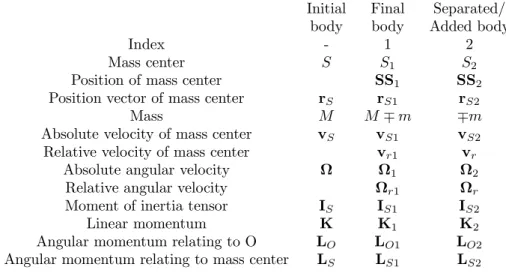
Depending on the velocity and the angular velocity of the separated body, the various cases of body motion are possible. In the following Tables some special cases of body separation are shown, together with the corresponding properties of the remainder body, calculated on the bases of (28) and (42).

Table 2. provides properties of the remainder body for the case when the initial body is in translation. Subcases for various absolute velocityv_S2 of mass center and absolute angular velocityΩ₂of the separated body are considered.

Table 2. Translation of the whole body vS = 0 Ω = 0

No. Separated body Remainder body

1 vS2= 0, Ω2= 0 vr1=−_M−m^m vr,

IS1Ω1k=SS₂×(vS1−v_S2)m

−IS2Ω2k.

2 v_S2= 0, Ω2= 0 v_r1=−_M−m^m v_r,

IS1Ω1k=SS₂×(vS1−v_S2)m.

3 v_S2= 0, Ω₂= 0 v_S1= _M−m^M v_S,

I_S1Ω₁k= _M−m^Mm SS₂×v_S

−I_S2Ω₂k.

4 vS2= 0, Ω2= 0 vS1= _M−m^M vS,

I_S1Ω₁k= _M−m^Mm SS₂×v_S. 5 v_S2= 0, Ω2k=−_IS2(M−m)^mM SS₂×v_r v_S1=v_S−_M−m^m v_r,

Ω₁= 0.

6 v_S2= ^M_mv_S, Ω₂= 0 v_S1= 0,

I_S1Ω₁k=−M(SS₂×v_S)

−I_S2Ω₂k.

7 v_S2= ^M_mv_S, Ω2k= _I^M_S

2(vS ×SS₂) v_S1= 0, Ω1= 0.

8 vS2=vS,(vr= 0) Ω2= 0 vS1=vS, IS1Ωr1k

=−IS2Ωrk.

In Table 3. the velocity and the angular velocity of the remainder body for the case when the initial body is rotating are shown. Subcases are considered with respect to various values of the relative velocity vr of mass center and the relative angular velocityΩrof the separated body.

Table 3. Rotating of the whole body vS = 0 Ω= 0

1 v_r= 0, Ω_r= 0 v_S1=Ω×SS₁−_M−m^m v_r, Ω_r1k= _I^M_S

1(SS₁×v_r)−^I_I^SS²1Ω_rk.

2 v_r= 0, Ω_r= 0 v_S1=Ω×SS₁, Ω_r1k=−^I_I^SS²1Ω_rk.

3 v_r= 0, Ω_r= 0 v_S1=Ω×SS₁,

Ω_r1= 0, Ω₁= Ω.

4 v_rSS₁, Ω_r= 0 v_S1=Ω×SS₁−_M−m^m v_r, Ωr1k=−^I_I^SS²1Ωrk.

5 v_S2=Ω×SS₂+v_r, v_S1=−_M−m^m v_S2,

Ω_r=−Ω,(Ω₂= 0) I_S1Ω₁k=I_SΩk−_M−m^Mm (SS₂×v_S2).

(22)

Table 3.

6 vr=^M−m_m (Ω×SS1), Ωr= 0 vS1= 0, Ωr1= _I^M_S

1

M−mm Ω(SS1)²+^I_I^S_S²

1Ωr.

7 v_r= 0, v_S1=Ω×SS₁−_M−m^m v_r,

IS2Ωrk=M(SS1×vr) +IS1Ωk Ωr1= 0, Ω1= Ω.

8 v_r=^M−m_m (Ω×SS₁), v_S1= 0, Ω_r= (^I_I^S_S¹

2 −^M(M−m)_m ^SS_IS2¹²)Ω Ω_r1= 0, Ω₁= Ω.

Table 4. Plane motion of the whole body v_S = 0 Ω= 0

1 vr=SS2×Ω,(vS2=vS), Ω2= 0 vr1=SS1×Ω, (vS1=vS), Ω₁=_I^I_S^S

1Ω−^I_I^SS²1Ω₂. 2 vr=SS2×Ω, Ω2= (IS/IS2)Ω vS1=vS, Ω1= 0.

3 vr=SS2×Ω, Ω2= 0 vS1=vS,

Ω1= (IS/IS1)Ω.

4 v_r=SS₂×Ω, Ωr= 0 v_S1=v_S,

Ω₁= Ω, Ω_r1= 0.

5 v_r= 0, Ω_r= 0 v_r1= 0, Ω_r1= 0.

Table 4. provides properties of the remainder body for the case when the whole body has the plane motion.

Analyzing the results in the Tables 2-4 the following is concluded:

1. If the relative velocity and the relative angular velocity of body separation are zero, the relative velocity and the relative angular velocity of the remainder body are also zero, independently of the type of motion of the initial body (see Table 2 case 4, Table 2 case 3 and Table 4 case 5). The absolute velocity of mass center of the remainder body is equal to the dragging velocity ofS₁ before body separation. The angular velocity of the remainder body is equal to the angular velocity of the initial body before separation.

2. If the motion of the initial body and of the separated body is translatory with velocityvS (the relative velocityvr is zero), the velocity of mass center of the remainder body is alsovS.This result was previously obtained by I.V. Meshchersky, 1896, for the continual mass variation of the translatory moving particle. Namely, due to the fact that the relative velocity of mass separation is zero, the reactive force is also zero and the equation of motion is the same as for the body without mass change.

3. If the motion of the initial body is translatory with the velocity v_S and the absolute velocity and the absolute angular velocity of separation of the body are zero, the absolute velocity of mass center of the remainder body differs from the velocity of the initial body. The velocity depends on the mass which is separated: for the higher value of separated massm i.e., for smaller value of the remainder mass, the velocity is higher. The solution of the Levi-Civita equation (Levi Civita, 1928)

v= Q

M, (45)

shows that if mass decreases the velocity of motion increases. Qis a constant which depends on the velocity properties of the system.

4. If the motion of the initial body is translatory, the relative angular velocity and the absolute angular velocity of the remainder body are equal (see Table 2).

(23)

3.3.2 Example: Separation of a part of the rotor

Fig.16. Model of the symmetrical rotor before body separation.

A symmetrically supported rotor, which is modelled as a shaft-disc system, is considered (see Fig.16). Mass of the disc isM.The mass centerSis in the geometric center of the disc. Mass of the shaft is negligible in comparison to the mass of the disc. The moment of inertia of the disc is IS for the axisz in mass center S. The rigidity of the shaft isc. The motion of the disc is in a planeOxy. The differential equations which describe the motion of the rotor are

Mx¨+cx= 0, My¨+cy= 0, I_Sψ¨+kψ˙ =M, (46) wherekis the damping coefficient andMis the torque.

The steady state solution for the third differential equation (46) is Ωb=M

k . (47)

The angular velocity depends on the external moment and damping of the system.

By introducing the complex deflectionzS =x+iy wherex, yare the coordinates of the mass centerS, i=√

−1is the imaginary unit andωw=

c/Mis the frequency of vibration, the differential equation of motion of mass center is

¨

z_S+ω²_wz_S = 0. (48)

For the initial conditions

x(0) =x_S0, y(0) =y_S0, x˙_S(0) =v_Sx0, y(0) =˙ v_Sy0, (49) the deflection of mass center yields

z_S = (A₀+iB₀) exp(iω_wt) + (C₀+iD₀) exp(−iω_wt), (50) where

A₀=1

2(x_S0+vSy0

ω_w ), B₀= 1

2(y_S0−vSx0

ω_w ), C₀=1

2(x_S0−v_Sy0

ω_w ), D₀= 1

2(y_S0+v_Sx0

ω_w ). (51)

The rotor center oscillates around the initial position of mass center.

(24)

Fig.17. Velocity distribution during separation: a) The position of mass center is such that∠ASS2=α, b)SS2 andAS are colinear.

If the rotor struck the fixed part of a stator inA(Fig.17a) at a momentt1, a part of the rotor is separated. The mass of the separated part ism, with mass centerS2

and the moment of inertia IS2 related to the axis in S2. The velocity ofS2 of the separated part is the sum of the dragging velocityv_S2d and the relative velocityv_r

vS2=vS2d+vr, where

v_S2d=

v_Sb² + (v_S2^S )²+ 2v_Sbv_S2^S sinα, sinγ= v_S2^S

v_S2dcosα, (52) with

v_S2^S = Ωb(SS2), and according to (50)

vSb=

˙

x²+ ˙y²=ωw

(C0−A0)²+ (B0−D0)²−2(C0−A0)(B0−D0) sin(2ωwt1), αis the angle betweenSS2 andSA. The dragging velocity

v_S2d=v_S2dT +v_S2dN, (53) has two components: the normal one, in theAS₂ direction

v_S2dN=v_S2dcos(β−γ), (54) and the tangential one, orthogonal to theAS2

v_S2dT =v_S2dsin(β−γ), (55) where

tanβ=SS2

R

sinα

(1−cosα). (56)

In the moment of contact between the rotor and the stator, the relative velocity and relative angular velocity of the separated body are

v_r=−v_S2dT, Ω_r=v_S2dT AS2

. (57)

(25)

Using the relations (28), (44) and (57) the relative velocity of the mass center of the remainder body and the relative angular velocity are calculated

v_r1= m

M−mv_S2dT, I_S1Ω_r1k=−I_S2vS2dT

AS₂ k+ m

M−mSS₂×v_S2dT. (58) The absolute velocity and angular velocity of the remainder rotor are

vS1 = vSb+Ωb×SS1+ m

M−mvS2dT, IS1Ω1ak = ISΩbk−IS2Ω2ak+ m

M−mSS₂²Ωbk

+ m

M−mSS2×vS2dT. (59)

For the special case whenα= 0andβ= 0,i.e., the mass center of the separated body is in theSAdirection (Fig.4b) and also the velocityv_Sb, the angleγare determined

sinγ= Ω_bSS₂

v_S2d, (60)

where

v_S2d=

v_b²+ (SS₂)²Ω²_b. (61) The separation of the body is with the relative velocity

v_r=Ω_b×SS₂, (62) and the relative angular velocity

Ωr= SS₂

AS2Ωb. (63)

The absolute velocity and the angular velocity of the remainder body are v_S1=v_Sb, Ω_1a= I_S

I_S1Ω_b−I_S2

I_S1Ω_b R

R−SS₂ = Ω_b(1−I_S2 I_S1

SS₂

R−SS₂), (64) whereRis the radius of the rotor. The angular velocity of the remainder body jumps to a lower value during separation: if the moment of inertia of the separated body is larger, the decrease of the angular velocity is higher.

For the special case when I_S1 = I_S2(SS₂/AS₂), the angular velocity of the remainder body is zero.

The velocityv_S1and angular velocityΩ_1arepresent the initial velocity and angular velocity for motion of the remainder body after separation.

Transient motion of the remainder body after separation The motion of the remainder body after separation is described with the following differential equations (M−m)¨x=X, (M−m)¨y=Y, IS1ψ¨+kψ˙ =M+cxSS1sinψ−cySS1cosψ, (65) whereXandY are the projections of the elastic force in the shaft

X=−c(x+SS1cosψ), Y =−c(y+SS1sinψ). (66) Introducing the notation

ω²= c

M−m, s=SS₁, k^∗= k IS1

, M^∗= M IS1

, p²= M−m IS1

, (67)

(26)

the differential equations (65) transform to

¨

x+ω²x = −sω²cosψ, y¨+ω²y=−sω²sinψ,

ψ¨+k^∗ψ˙ = M^∗+sp²ω²xsinψ−sp²ω²ycosψ. (68) Due to shortness of the time, the position variation of the body is small (x <1, y <1, ψ <1). The linearized differential equations (68) are

¨

x+ω²x = −sω²,

¨

y+ω²y = −sω²ψ,

ψ¨+k^∗ψ˙ = M^∗−syω²p². (69) The first differential equation in the system (69) is independent and the solution for the initial conditions x(0) = x(t₁) (see (50)) and x(0) =˙ v_S1x, where v_S1x is the projection in the x direction of the velocity ofS₁ of the remainder body after separation, are obtained

x= (x_S1+s) cosωt+v_S1x

ω sinωt−s, (70)

For the initial conditions y(0) = yS1(t1), y(0) =˙ vS1y, ψ(0) = ψ(t1) = ψ₀ and ψ(0) = Ω˙ _1a,the displacement in they direction and the angular velocityψ˙ are

y = s

k^∗(Ω−Ω_1a)−sψ₀−s(Ωt)− sω²

(ω²+k^∗2)k^∗(Ω−Ω_1a) exp(−k^∗t) +[v_S1y

ω + sω

ω²+k^∗2(Ω1a+ Ωk^∗2 ω²)] sinωt +[(y0+sψ₀)−(Ω−Ω1a) sk^∗

ω²+k^∗2] cosωt. (71)

and ψ˙ = Ω−(Ω−Ω_1a) exp(−k^∗t). (72)

For the initial velocity and the angular velocity (64), where Ωb = Ω and SS2 = R−SS₁,the transient motion yields

y = Ω

k^∗ I_S2 IS1

(R−s)−sψ₀−s(Ωt)− ω²Ω (ω²+k^∗2)k^∗

I_S2 IS1

(R−s) exp(−k^∗t) +[vS1y

ω + sωΩ

ω²+k^∗2(1−IS2

I_S1 R−s

s +k^∗2

ω²)] sinωt +[y₀+sψ₀−ΩI_S2

IS1

k^∗(R−s)

ω²+k^∗2 ] cosωt, (73)

and

ψ˙ = Ω(1−I_S2 I_S1

R−s

s exp(−k^∗t)). (74)

During separation the angular velocity starts withΩ1aand tends to the steady state angular velocityΩ,which depends on the moment and damping acting on the rotor:

the higher the damping, the lower the angular velocity. If the torque is larger, the angular velocity is also higher.

Mass center of the remainder body moves with the velocity (sΩ), which depends on the properties of the system and the distance between mass center and rotation center of the remainder body: the smaller the parameter s, the motion is slower. If the velocity is significant, the remainder body impacts the fixed stator, but if the velocity is smaller, the mass center tends to its steady state position.

Dynamics of Mass Variable System Cvetityanin Lívia, PhD MTA doktori értekezés Szeptember 2012