The impact of Covid-19 on agriculture: evidence from oats and wheat markets

(1)

Introduction

The recent Covid-19 pandemic has spread from one coun- try to another, having its origin in Wuhan-Hubei, China (Liu et al., 2020). The total cases globally amount to over 51 mil- lion people (November 2020), showing the cruel face of this pandemic (WHO, 2020). The case of Covid-19 is unique, differing in many ways from previous disease spreads, such as the severe acute respiratory syndrome (SARS) spread in 2003 (Wilder-Smith et al., 2020). The rapid spread of the Covid-19 disease in a worldwide context has spread fear globally.

The Covid-19 pandemic has changed the dynamics of the overall economy, impacting many fields, including the agricultural sector, as the fear spread by the Covid-19 has led to an excess demand, of the major commodities of the primary sector. The lockdown measures made the matters worse, as the fear of a long-term quarantine had an impact on the consumers. This led to a phenomenon, known as “panic buying”, where consumers emptied the shelves in the supermarkets (Sim et al., 2020).

The situation following the Covid-19 lockdown measures was unprecedented. Covid-19 disrupted the agricultural sector in many ways. To begin with, government organisa- tions posed interruptions in the acquirement of nourishment grains. This included lockdown measures, panic spread, leading to lack of labourers to collect the crops, deficiency of drivers in the transportation area, disturbances in the assortment of harvests from the homesteads by private deal- ers. Moreover, the export restrictions and other trade policy measures that were introduced following the Covid-19 crisis made the situation even worse (Laborde et al., 2020).

Since in many countries the retail markets continued to function during the Covid-19 pandemic, in fear of the lockdown measures and long-term quarantine, consumers got into a state of “panic buying”, emptying the shelves in the supermarkets (Sim et al., 2020), leading to a an increase in prices, caused by the excess demand. The excess demand and the decreased supply led to an important effect in the prices of the agricultural commodities, out of which oats and

wheat turned out to be very important ones. Our aim is to depict this effect on the prices of oats and wheat.

In the presence of such post-apocalyptic situations, stock traders and investors adapt their trading behaviour.

More precisely, traders swap from other stocks, to the assets considered more stable or more profitable. Since the market demand for agricultural commodities increased, con- sequently, the values of these stocks also increased, and this effect is depicted in the present paper’s results. In this paper, using relevant econometric techniques, we capture the impact of the Covid-19 spread on two important commodities from the agricultural sector, namely oats and wheat. The present paper contributes to the literature in the following ways: (a) it is the first attempt, to the best of our knowl- edge, to investigate the effect of the Covid-19 spread and the lockdown measures on certain agricultural commodities, using global data; (b) it proposes an alternative approach to the examination of the economic effect of the crisis on the agricultural sector, based on a financial framework; and (c) it provides a robustness analysis of the findings based on out- of-sample forecasting accuracy measures.

The paper is structured as follows: Section 2 presents the literature review; Section 3 describes the methodology used, Section 4 presents the empirical results and finally, Section 5 concludes.

Literature Review

To begin with, Bonny (1998) studied a number of factors that may play a role in agriculture, including crises and changing demand. Based on the results, farming ought to become fine-tuned and environmentally harmless, multi- form and multi-functional, with its production model being diversified and adaptive.

Agricultural commodities have special characteristics, differing from other commodities. For instance, they are known to converge faster to long run equilibrium than other commodities, e.g. metal and energy commodities. Moreo- Theodoros DAGLIS*, Konstantinos N. KONSTANTAKIS* and Panayotis G. MICHAELIDES*

The impact of Covid-19 on agriculture: evidence from oats and wheat markets

The Covid-19 pandemic has changed the dynamics of the overall economy, impacting many fields, including the agricultural sector. In this paper, we examine two important commodities of the agricultural sector, namely oats and wheat, during the Covid-19 spread and the lockdown measures. Using relevant time series specifications, we establish a hypothesis regarding the effect of the Covid-19 pandemic on these two commodities. Based on our findings, the commodities were affected by the Covid-19 spread and moreover, the Covid-19 confirmed cases provide useful information for the prediction and forecasting of these values. Our findings are robust, since the out-of-sample forecasting accuracy of the alternative model employed, that explicitly incorporates the pandemic induced by the Covid-19 disease, is superior to the baseline model.

Keywords: Covid-19, agriculture, oats, wheat, commodities JEL classifications: C22, C58, C50, C51

* National Technical University of Athens, School of Applied Mathematics and Physics. 9 Ir. Politechniou Str, Athens-157 72, Greece. Corresponding author:

theodagl4@gmail.com.

Received: 20 July 2020, Revised: 16 September 2020, Accepted: 20 September 2020.

(2)

ver, a spillover effect among agricultural commodities may be included, as has been shown in the past (Vandone et al., 2018). That is why oats and wheat may be linked, as many products require both of them, for their production, and moreover they are an important and basic means of diet.

More interestingly, it has been shown that stock markets exhibit a great impact on agricultural price dynamics during extreme movements. Such movements occurred during the 2007–2008 financial crisis, highlighting a potential influence of financial markets on the financialisation of commodities (Aït-Youcef, 2019). As for wheat, it has been shown that wheat prices exhibit a negative and statistically significant leverage effect (Sadorsky, 2014). This indicates that negative residuals tend to decrease the variance of the commodity, stabilising its value.

Ben Amar et al. (2020) argue that there is a strong effect of the Covid-19 crisis on various stocks and commodities, leading to spillovers. The export restrictions and other trade policy measures, following the Covid-19 crisis, were thought to increase global food prices, with consequences including the exacerbation of hunger and income losses for producers in export-restricting countries (Laborde et al., 2020).

Methodology

In order to econometrically investigate (non-)causality between the Covid-19 confirmed cases and agricultural prices, we will make use of the state of the art step-by-step (non-) causality test, introduced by Dufour and Renault (1998) and extended by Dufour et al. (2006). In this context, following standard time series literature (Hamilton, 1994), before turning to (non-)causality testing, we examine the level of integration of the time series that enter our analysis using the Phillips–Perron (1988) unit root test. More specifically, the hypothesis tested for the Phillips–Perron test is that the time series do not have a unit root. In addition, in case of integrated of degree one time series, i.e. I(1), we also test for the potential existence of long-run relationships among the variables, using the popular Johansen (1990) cointegration test, and the hypothesis tested is that the time series are not cointegrated. Finally, the optimal lag length of the time series variables was investigated using the Schwartz-Bayes information criterion (SBIC).

We should note that in case of non-stationarity (existence of unit root), the statistical properties of the time series are time dependent. This, could end up in misleading results. Moreover, co-integration is the case in which two or more time series have a long-term relationship that must be included in the model. That is why, in cases of co-integration, an error term must be included in the model. More specifically, the Johansen co-integration test is robust against non-normality whereas heteroscedasticity may have a minor effect on it.

Additionally, in order to cross validate the fact that the Covid-19 confirmed cases are causal and thus have predictive ability on the agricultural commodities, we will also make use of forecasting strategies. In detail, using a Vector autoregressive model as a baseline, we will investigate whether

an alternative specification that could also incorporate the information provided by the Covid-19 confirmed cases as an exogenous variable, outperforms the forecasting accuracy of the baseline model. To do so, three distinct measure of forecasting accuracy are used, namely the mean absolute error (MAE), the mean absolute percentage error (MAPE) and the root mean square forecasting error (RMSFE), to investigate the magnitude of the predictive power of Covid-19 spread on the agricultural commodities.

In what follows, we offer a brief outline of the techniques and procedures used in this work.

As a first step, we check for the potential existence of unit roots in our time series, using relevant unit root tests. More analytically, we implement the Phillips–Perron unit root test.

The null hypothesis of the test is that the time-series contain a unit root. In case of I(1) variables, we test for cointegration among the time-series. If cointegrating relationships are present, Error Correction Terms (ECM) have to be included in the model. In this work, we implement the Johansen (1988) test.

As a next step, we investigate (non-)causality between the Covid-19 confirmed cases and the agricultural commodities, using (non-)causality test. In order to study the exact timing pattern of the causality relationship, we make use of the state-of-the-art step-by-step causality introduced by Dufour and Renault (1998) and extended by Dufour et al.

(2006).

Based on recent advancement of the related literature of causality, other non-causality tests (for instance Granger non-causality test) fail to unveil the potential timing pattern of a causal relationship. In this context, in a seminal paper in Econometrica, Dufour and Renault (1998) introduced the notion of step-by-step or short-run causality based on the idea that two time series X_t and Y_t could interact in a causal scheme via a third variable Z_t. More precisely, despite the fact that X_t could not cause Y_t one period ahead, it could cause Z_t one period ahead i.e. Z_t+1, and Z_t could cause Y_t two periods ahead i.e. Y_t+2. Therefore, X_t → Y_t+2, even though X_t ↛ Y_t+1. For testing the step by-step causality, consider the following VAR (p) model:

(1)

where: Y_t is an (1×m) vector of endogenous variables, a is a (1×m) vector of constant terms; X_t is a vector of exogenous variables and u_t is a (1×m) vector of error terms such that where I is the identity matrix. The lags in the baseline model are selected using the Schwartz-Bayes Information criterion (SBIC).

Following Dufour et al. (2006), the model described in (1) corresponds to horizon h=1. In order to test for the existence of non-causality in horizon h, the procedure continuous in the same context.

Vector autoregressive (VAR) is a model used to capture the linear interdependencies among multiple time series.

Each variable in the VAR model, has an equation explaining its evolution based on its own lagged values, the lagged values of the other model variables, and an error term. A VAR model of order p, with exogenous variables is structured as follows:

(3)

(2)

where n is the number of the endogenous variables (y_i,t) of the model, c_i are the fixed terms, p is the lag order of the endogenous variables and e_i,t are the error terms of each equation of the model, as before. In the case of exogenous variables, k is the number of the independent or exogenous variables of the model (x_i,t) and q is the lag order of the exogenous variables. In case of co-integration between the variables, error correction term must be included in the model. In such a case, a Vector Error Correction Model (VECM) should be employed instead.

In this paper, we make use of the so-called Schwartz- Bayes Information criterion (SBIC) introduced by Schwarz (1978), because it is an optimal selection criterion when used in finite samples. We used the SBIC criterion for order and lag selection when needed. Additionally, in order to cross validate our results, we make use of the AIC (Akaike, 1973), Hannan-Quinn (Hannan and Quinn, 1979) and FPE (Ljung, 1999) criteria.

We also make use of the following forecasting accuracy measures: the mean absolute error (MAE), the mean absolute percentage error (MAPE) and the root mean square forecast error (RMSFE). In general, the smaller the values of each forecasting criterion, the better the forecasting value.

A model’s MAE for forecast horizon h is given by the following:

(3) where: ℎ is the forecast horizon of the model, 𝐹_𝑡 are the out- of-sample forecasted values of the model, and 𝐴_𝑡 are the actual values. The smaller the MAE values of a model the better its forecasting ability. However, one of the main disad- vantages of the MAE is the fact that is has no standard scale and it is not as comparable as a percentage. To overcome this problem, we will also base our analysis on MAPE.

A model’s MAPE is given by the expression:

(4)

MAPE is measured as a percentage change and again, the smaller the MAPE of a model, the better its predictive ability.

The RMSFE is used to measure the forecasting error dis- tribution. It is given by the expression:

(5) Overall, both in MAE and RMSE measures, we get the mean error or the root of the mean error of a forecast. There-

fore, the values of the measures depend on the forecasted values. The MAPE measure, on the other hand, is measured as a percentage change. That is why we can compare its suc- cess on different and even unrelated datasets.

Empirical Analysis

The data used in the present paper are the global confirmed cases of Covid-19 in daily format and were down- loaded by the Johns Hopkins University database and span the period 22 January 2020 until 2 June 2020. The confirmed cases were transformed into logarithms. Moreover, we used two major commodities of the agricultural sector, namely oats and wheat, adjusted close prices, derived from finance.yahoo in daily frequency, and span also the period 22 January 2020 until 2 June 2020. The two agricultural commodities were chosen based on the fact that they were considered among the most important and multipurpose agricultural commodities, and moreover, because these commodities were used (primarily) for the same reasons, namely for food source of animals and food source or bev- erage for people.

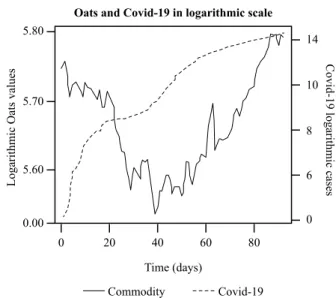
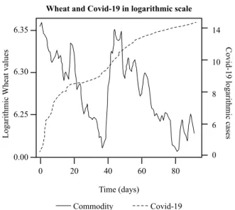
The descriptive statistics of the time series are depicted in Table 1. Furthermore, the plots of the logarithmic confirmed Covid-19 cases and the two logarithmic values of the commodities are depicted in Figures 1 & 2.

Figures 1 & 2 provide graphical evidence of the impact of the Covid-19 spread on the agricultural sector, a fact that needs to be investigated thoroughly using econometric

Table 1: Descriptive statistics of the time series.

Variable Mean Standard

Deviation Min Max Log_Confirmed

Covid-19 cases 5.5821 1.0203 2.7443 6.8047 Log_Oats 2.4604 0.0304 2.4035 2.5179 Log_Wheat 2.7290 0.0183 2.6974 2.7638 Source: Authors’ elaboration

Oats and Covid-19 in logarithmic scale

Time (days)

Logarithmic Oats values Covid-19 logarithmic cases

0 0.00 5.60 5.70 5.80

0 8 6 10 14

80

20 40 60

Commodity Covid-19

Figure 1: Log confirmed Covid-19 cases and log values of oats.

Source: Authors’ elaboration

(4)

methods. We set out the hypothesis tested, that the Covid-19 spread, affects the prices of these two commodities.

We make use of step-by-step causality in order to iden- tify whether the Covid-19 spread “causes” the values of the two commodities. As a next step, we test the contribution of the information derived by the Covid-19 confirmed cases on the forecasting of the aforementioned commodities. To do so, we make use of two econometric models in the form of Vector autoregressive model (since there is connec- tion among the two prices). The first model, declared as the baseline, is a Vector autoregressive model only with endogenous variables (the two commodity prices) and an alternative model being the same with the baseline, aug- mented with one exogenous variable, the Covid-19 global confirmed cases. The comparison of these two models, in terms of forecasting ability, will unveil a possible contribution of the exogenous variable on the forecasting of the two commodity prices.

A first step in every econometric modelling is the unit root test (Phillips–Perron unit root test are used here). The results are depicted in Table 2.

As stated in the methodology section, the Phillips–Perron null hypothesis is that the time series have a unit root. If we reject the null hypothesis for p-value less than 0.1, it means that the specific time series does not have unit root.

Since the results in Table 2 show that the Covid-19 p-value is smaller than 0.1, we reject the null hypothesis and therefore, the Covid-19 confirmed cases do not have a unit root, meaning that the time series is stationary. Moreo- ver, oats and wheat have p-values greater than 0.1, so, for these time series, we cannot reject the Phillips–Perron null hypothesis, and therefore, these timeseries are I(1). In the case of the non-stationary variables (oats and wheat), the presence of co-integration should be tested.

The results of the co-integration test are depicted in Table 3, indicating that there are no cointegration relationships among the timeseries since we cannot reject the rank r = 0. Since the Covid-19 cases are I(0), and the I(1) variables are not co-integrated, in such case, no error correction

term should be included in the econometric models, but first difference transformation must take place at least for the I(1) variables. The next step is the use of the step-by-step causality tests (Table 4).

Again, as stated in the methodology section, the null hypothesis of the Wald test in the step-by-step causality is that the exogenous variable does not step-by-step cause the endogenous one. If the p-value of the Wald test is less than 0.1, then, we may infer that the null hypothesis is rejected and therefore, the independent variable step-by-step causes the endogenous one. The results in Table 4 indicate that the Covid-19 variable “causes” the commodities in multiple steps, since in these steps the results of the Wald test reject the null hypothesis of non-causality.

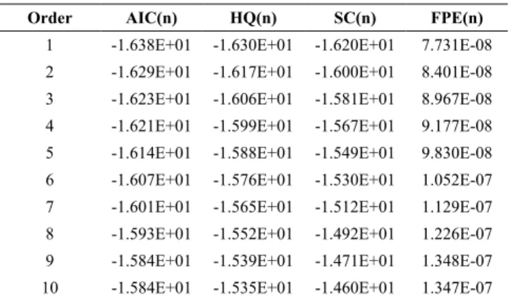
Having shown that the Covid-19 spread “causes” the values of the two commodities, and therefore it provides useful information for their interpretation and their modelling, we will test if the Covid-19 spread contributes to their forecasting. To do so, we first decide for the lag order of the econometric models (baseline and alternative), based on the SBIC criterion. The results are depicted in Table 5 & 6.

Based on the results, the AIC, SBIC, HQ and FPE criteria indicate the lag order 1 as the most appropriate for both models since the smallest criteria values indicate the most appropriate lag order. In this case, the lag order of the baseline and alternative model will be selected to be equal to one (1).

The baseline model incorporated one lag order for each endogenous variable (oats and wheat). Using out of sample forecast with a fixed window, for horizon h=1,2,…,10, we forecast for two weeks, based on the business calendar. Then, we employ the same model incorporating as exogenous variable the logarithm of global confirmed Covid-19 cases and test again the forecasting ability of this alternative model.

Wheat and Covid-19 in logarithmic scale

Time (days)

Logarithmic Wheat values Covid-19 logarithmic cases

0 0.00 6.25 6.30 6.35

0 8 6 10 14

80

20 40 60

Commodity Covid-19

Figure 2: Log Confirmed Covid-19 cases and log values of wheat.

Table 2: Phillips–Perron unit root test results for the time series.

Variable PP test P-value Integration term Log_Confirmed Covid-19 cases 0.010 I(0)

Log_Oats 0.923 I(1)

Log_Wheat 0.393 I(1)

Table 3: Johansen Cointegration test results for the I(1) time series.

Rank Test 10pct 5pct 1pct

r<=1 2.140 6.50 8.180 11.650

r=0 7.850 12.910 14.90 19.190

Table 4: Step-by-step causality results for the case of oats and wheat.

Oats Wheat

Wald test P-value Order Wald test P-value Order

3.178 0.079 16 3.582 0.063 18

3.113 0.082 18 - - -

5.139 0.027 19 - - -

3.873 0.053 21 - - -

2.660 0.108 24 - - -

(5)

model with exogenous variable Covid-19 confirmed cases) than the respective accuracy measures’ values for the case of the VAR (alternative model without exogenous variable).

This implies that Covid-19 provides useful information for the forecasting of the values of oats and wheat.

Finally, using the impulse – response function, and more precisely, the orthogonalised impulse responses, the results We then compare the two models in terms of their forecast-

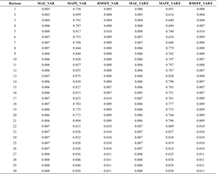
ing ability, based on the MAE, MAPE, RMSFE. The results are depicted in Tables 7 & 8.

The results above show that the alternative model is better in terms of forecasting ability than the baseline, for the two commodities analysed, since MAE, MAPE and RMSFE values are smaller for the case of the VARX (alternative Table 5: Results of the AIC, SBIC, Hannan-Quinn and FPE criteria for the case of the Baseline model.

Order AIC(n) HQ(n) SC(n) FPE(n)

1 -1.638E+01 -1.630E+01 -1.620E+01 7.731E-08 2 -1.629E+01 -1.617E+01 -1.600E+01 8.401E-08 3 -1.623E+01 -1.606E+01 -1.581E+01 8.967E-08 4 -1.621E+01 -1.599E+01 -1.567E+01 9.177E-08 5 -1.614E+01 -1.588E+01 -1.549E+01 9.830E-08 6 -1.607E+01 -1.576E+01 -1.530E+01 1.052E-07 7 -1.601E+01 -1.565E+01 -1.512E+01 1.129E-07 8 -1.593E+01 -1.552E+01 -1.492E+01 1.226E-07 9 -1.584E+01 -1.539E+01 -1.471E+01 1.348E-07 10 -1.584E+01 -1.535E+01 -1.460E+01 1.347E-07 Source: Authors’ elaboration

Table 6: Results of the AIC, SBIC, Hannan-Quinn and FPE criteria for the case of the Alternative model.

Order AIC(n) HQ(n) SC(n) FPE(n)

1 -2.186E+01 -2.172E+01 -2.151E+01 3.196E-10 2 -2.172E+01 -2.147E+01 -2.110E+01 3.702E-10 3 -2.160E+01 -2.124E+01 -2.071E+01 4.190E-10 4 -2.152E+01 -2.105E+01 -2.036E+01 4.564E-10 5 -2.167E+01 -2.110E+01 -2.025E+01 3.956E-10 6 -2.164E+01 -2.096E+01 -1.995E+01 4.108E-10 7 -2.155E+01 -2.076E+01 -1.959E+01 4.582E-10 8 -2.142E+01 -2.053E+01 -1.921E+01 5.289E-10 9 -2.129E+01 -2.029E+01 -1.881E+01 6.196E-10 10 -2.127E+01 -2.017E+01 -1.852E+01 6.553E-10 Source: Authors’ elaboration

Table 7: MAE, MAPE and RSMFE forecasting accuracy of the VAR (baseline model) and VARX (alternative model) for the case of oats.

Horizon MAE_VAR MAPE_VAR RMSFE_VAR MAE_VARX MAPE_VARX RMSFE_VARX

1 0.019 1.087 0.019 0.019 1.050 0.019

2 0.044 1.032 0.050 0.044 1.021 0.050

3 0.033 1.062 0.041 0.033 1.025 0.042

4 0.027 1.098 0.036 0.026 1.032 0.036

5 0.022 0.982 0.032 0.021 0.973 0.032

6 0.018 1.227 0.029 0.018 1.044 0.030

7 0.017 1.236 0.027 0.016 1.047 0.027

8 0.015 1.237 0.026 0.015 1.048 0.026

9 0.015 1.229 0.024 0.014 1.047 0.024

10 0.015 1.212 0.024 0.015 1.045 0.024

11 0.015 1.207 0.023 0.014 1.045 0.023

12 0.015 1.182 0.023 0.014 1.039 0.023

13 0.015 1.173 0.023 0.015 1.037 0.022

14 0.015 1.176 0.022 0.014 1.038 0.022

15 0.014 1.267 0.021 0.013 1.079 0.021

16 0.014 1.257 0.021 0.013 1.076 0.021

17 0.013 1.257 0.020 0.013 1.074 0.020

18 0.013 1.199 0.020 0.012 1.061 0.019

19 0.013 1.192 0.020 0.013 1.059 0.020

20 0.013 1.188 0.020 0.013 1.058 0.019

21 0.013 1.194 0.019 0.012 1.059 0.019

22 0.013 1.210 0.019 0.012 1.061 0.018

23 0.012 1.207 0.018 0.012 1.059 0.018

24 0.012 1.206 0.018 0.012 1.058 0.018

25 0.013 1.200 0.018 0.012 1.057 0.018

26 0.012 1.176 0.018 0.012 1.051 0.018

27 0.012 1.201 0.018 0.011 1.055 0.017

28 0.012 1.191 0.017 0.011 1.053 0.017

29 0.012 1.187 0.018 0.012 1.052 0.017

30 0.012 1.172 0.017 0.011 1.048 0.017

(6)

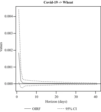
indicate that the effect of Covid-19 on oats is positive, as depicted in Figure 3, since the orthogonalised impulse- response function is positive, and statistically significant, since the 95% confidence intervals do not include zero. This means that a unit shock in the Covid-19 spread, will lead to an increase in oats prices. In the same context, the effect of the Covid-19 variable on wheat is positive, as depicted in Figure 4, since again the orthogonalised impulse-response function is positive, but is statistically significant only in the beginning of the shock, since the 95% confidence intervals do not include zero in the beginning, but later on, they include it, and therefore, it is not statistically significant.

Note that for the impulse-response function plots, the Covid- 19 cases are in logarithms, for graphical reasons.

In an attempt to minimise the spread of the coronavirus, most economies and policy makers have taken extreme lockdown measures that adversely affect the overall micro- economic, macroeconomic and financial conditions in a global scale. As a result, the lockdown caused a massive shock that could lead to inflation. Many governments have posed interruptions in the acquirement of nourishment grains and/or imposed export restrictions and other trade policy measures (Laborde et al., 2020). These, led to the intensification of shocks in the agricultural sector. Moreo-

ver, due to “panic buying”, as a result of the fear of the lockdown measures and long-term quarantine, consumers emptied the shelves in the supermarkets (Sim et al., 2020), leading to a greater increase in the prices, caused by the excess demand. The excess demand and the decreased supply led to an important effect in the prices of oats and wheat. As shown by our results, the impact of Covid-19 on oats and wheat is positive, meaning that Covid-19 increases the price of both commodities.

At this point, we should highlight the variability in the data used in the present paper. More analytically, the global Covid-19 cases are in an aggregate format and hide probable heterogeneity. This means that different regions across the globe adopt different measures, and faced different Covid-19 cases. We capture the aggregate dynamics, but there could be different effects in different regions. As an extension of the present paper, one could examine the impact of Covid-19 around the world on different regions through economic and financial framework. Last but not least, in some countries, the actual numbers are questionable due to misreporting.

Our findings are in accordance with the existing literature since it has been shown that stock markets exhibit a great impact on agricultural price dynamics during extreme movements, such as during financial crises (Aït-Youcef, 2019).

Table 8: MAE, MAPE and RSMFE forecasting accuracy of the VAR (baseline model) and VARX (alternative model) for the case of wheat.

Horizon MAE_VAR MAPE_VAR RMSFE_VAR MAE_VARX MAPE_VARX RMSFE_VARX

1 0.005 0.756 0.005 0.006 0.891 0.006

2 0.003 0.699 0.004 0.003 0.616 0.004

3 0.004 0.741 0.004 0.004 0.640 0.004

4 0.006 0.787 0.008 0.006 0.696 0.007

5 0.008 0.817 0.010 0.008 0.740 0.010

6 0.007 0.753 0.009 0.007 0.634 0.009

7 0.007 0.768 0.009 0.007 0.648 0.008

8 0.007 0.844 0.008 0.006 0.779 0.008

9 0.006 0.840 0.008 0.006 0.765 0.008

10 0.006 0.828 0.008 0.006 0.747 0.007

11 0.006 0.857 0.008 0.006 0.797 0.008

12 0.006 0.855 0.008 0.006 0.787 0.007

13 0.007 0.875 0.008 0.006 0.820 0.008

14 0.006 0.830 0.008 0.006 0.790 0.007

15 0.006 0.827 0.007 0.006 0.783 0.007

16 0.006 0.815 0.007 0.005 0.751 0.007

17 0.007 0.823 0.010 0.007 0.761 0.009

18 0.007 0.783 0.009 0.006 0.777 0.009

19 0.006 0.775 0.009 0.006 0.753 0.009

20 0.006 0.773 0.009 0.006 0.744 0.009

21 0.006 0.804 0.009 0.006 0.796 0.009

22 0.007 0.815 0.010 0.007 0.809 0.010

23 0.007 0.828 0.010 0.007 0.827 0.010

24 0.007 0.832 0.010 0.007 0.828 0.010

25 0.007 0.828 0.010 0.007 0.819 0.010

26 0.007 0.828 0.010 0.007 0.814 0.010

27 0.008 0.836 0.011 0.008 0.825 0.011

28 0.008 0.846 0.011 0.008 0.838 0.011

29 0.008 0.848 0.011 0.008 0.838 0.011

30 0.008 0.850 0.011 0.008 0.838 0.011

(7)

Covid-19 -> Oats

Horizon (days) 0

-0.001 0.000 0.001 0.002 0.003 0.004

40

10 20 30

OIRF 95% CI

Values

Figure 3: Impulse response function for the case of oats.

Covid-19 -> Wheat

Horizon (days) 0

0.000 0.001 0.002 0.003 0.004

40

10 20 30

OIRF 95% CI

Values

Figure 4: Impulse response function for the case of wheat.

Moreover, it has been also shown that there is a strong effect of the Covid-19 crisis on various stocks and commodities, leading to spillovers (Ben Amar et al., 2020). Finally, Laborde et al. (2020) have already argued that the export restrictions and other trade policy measures, following the Covid-19 crisis, would increase global food prices (Laborde et al., 2020).

Conclusions

The paper investigated the early impact of Covid-19 on the prices of oats and wheat in the global market. By using relevant time series specifications, we established a hypothesis regarding the effect of Covid-19 on the prices of these commodities. The evidence supported the stated hypotheses , as based on our findings, the Covid-19 spread

“step-by-step caused” prices of oats and wheat. Further- more, the Covid-19 spread provides useful information for the forecasting of these commodities, as shown by the forecasting comparison of the baseline and alternative model, indicated by the forecasting criteria MAE, MAPE and RMSFE. Our findings are robust, since the out-of-sample forecasting accuracy of the alternative model employed, that explicitly incorporates the pandemic induced by the Covid-19 disease, is superior to the baseline model.

Our findings imply that the Covid-19 spread not only contributes with statistically significant information to the modelling of both agricultural commodities but also increases the forecasting ability of these commodities in the 22/01 – 02/06 time period (2020). This fact shows the great impact of Covid-19 on the agricultural sector worldwide, affecting the total economy.

We hope our work can serve as a basis for more sophisti- cated models, testing for other factors that could play a sig-

nificant role in forecasting the prices of various agricultural commodities.

Acknowledgement

We are indebted to the anonymous Referees and the Edi- tor-in-Chief of Studies in Agricultural Economics for their constructive feedback.

References

Aït-Youcef, C. (2019): How index investment impacts commodities: A story about the financialization of agricultural commodities. Economic Modelling, 80, 23–33. https://doi.org/10.1016/j.

econmod.2018.04.007

Akaike, H. (1973): Information theory and an extension of the maximum likelihood principle. IN Petrov, B.N. and Csáki, F.

(eds.): 2nd International Symposium on Information Theory, Tsahkadsor, Armenia, USSR, September 2-8, 1971, Budapest:

Akadémiai Kiadó, 267–281.

Ben Amar, A., Belaid, F., Ben Youssef, A. Chiao, B. and Gues- mi, K. (2020): The Unprecedented Equity and Commod- ity Markets Reaction to COVID-19. Available at SSRN.

https://doi.org/10.2139/ssrn.3606051

Bonny, S. (1998): Prospects for Western agriculture during a period of crisis, changing demand, and scientific progress: a case study of France. Technology In Society, 20 (2), 113–130.

https://doi.org/10.1016/S0160-791X(98)00002-5

Dufour, J.-M., Pelletier, D., and Renault, E. (2006): Short run and Long run Causality in Time series: Inference. Journal of Econometrics, 132 (2), 337–362. https://doi.org/10.1016/j.

jeconom.2005.02.003

Dufour, J.-M. and Renault, E. (1998): Short-run and long-run causality in time series: theory. Econometrica, 66 (5), 1099–1125.

https://doi.org/10.2307/2999631

(8)

Hamilton, J.D. (1994): Time Series Analysis, Princeton University press.

Hannan, E.J. and Quinn, B.G. (1979): The Determination of the order of an autoregression. Journal of the Royal Statistical Society. Series B: Statistical Methodology, 41 (2), 190–195.

https://www.jstor.org/stable/2985032

Johansen, S. (1988): Statistical analysis of cointegration vectors.

Journal of Economic Dynamics and Control, 12 (2–3), 231–

254. https://doi.org/10.1016/0165-1889(88)90041-3

Johansen, S. and Juselius, K. (1990): Maximum likelihood estima- tion and inference on cointegration-with applications to the demand for money. Oxford Bulletin of Economics and Statistics, 52 (2), 169–210. https://doi.org/10.1111/j.1468-0084.1990.

mp52002003.x

Laborde, D., Mamun A. and Parent, M. (2020): Documentation for the COVID-19 Food Trade Policy Tracker: Tracking Gov- ernment Responses Affecting Global Food Markets during the COVID-19 Crisis. Retrieved from: https://www.ifpri.org/

project/covid-19-food-trade-policy-tracker (Accessed in May 2020).

Ljung, L. (1999): System Identification: Theory for the User. Upper Saddle River, NJ, Prentice-Hall PTR, Sections 7.4 and 16.4.

https://doi.org/10.1109/MRA.2012.2192817

Phillips, P.C.B. and Perron, P. (1988): Testing for a Unit Root in Time Series Regression. Biometrika, 75 (2), 335–346.

https://doi.org/10.1093/biomet/75.2.335

Sadorsky, P. (2014): Modeling volatility and correlations between emerging market stock prices and the prices of copper, oil and wheat. Energy Economics, 43, 72–81. https://doi.org/10.1016/j.

eneco.2014.02.014

Schwarz, G.E. (1978): Estimating the dimension of a model.

Annals of Statistics, 6 (2), 461–464. https://doi.org/10.1214/

aos/1176344136

Sim, K., Chua, H., C., Vieta, E. and Fernandeza, G. (2020): The anatomy of panic buying related to the current COVID-19 pandemic. Psychiatry Research, 288, 113015. https://doi.

org/10.1016/j.psychres.2020.113015

Vandone, D., Peri, M., Baldi, L. and Tanda, A. (2020): The impact of energy and agriculture prices on the stock performance of the water industry. Water Resources and Economics, 23, 14–27.

https://doi.org/10.1016/j.wre.2018.02.002

WHO - World Health Organization (2020): Coronavirus disease 2019 (COVID-19), Situation Report – 51. Retrieved from:

https://apps.who.int/iris/handle/10665/331475 Accessed in June 2020.

Wilder-Smith, A., Chiew, C.J. and Lee, V.J. (2020): Can we contain the COVID-19 outbreak with the same measures as for SARS?

The Lancet infectious diseases, Personal View, 20 (5), 1–6.

https://doi.org/10.1016/S1473-3099(20)30129-8