Forecasting exchange rates of major currencies with long maturity forward rates

Forecasting exchange rates of major currencies with long maturity forward rates

Zsolt Darvas^a and Zoltán Schepp^b

aBruegel and Corvinus University of Budapest, e-mail: zsolt.darvas@uni-corvinus.hu

bUniversity of Pécs, e-mail: schepp.zoltan@ktk.pte.hu March 30, 2020

Abstract

This paper presents unprecedented exchange rate forecasting results based upon a new model which approximates the gap between the fundamental equilibrium exchange rate and the actual exchange rate with the long-maturity forward exchange rate. The theoretical derivation of our forecasting equation is consistent with the monetary model of exchange rates. Our model outperforms the random walk in out-of-sample forecasting of twelve major currency pairs in both short and long horizons forecasts for the 1990-2020 period. The results are robust for all sub-periods with the exception of years around the collapse of Lehman Brothers in September 2008. Our results are robust to alternative model specifications, single equation and panel estimation, recursive and rolling estimation, and alternate data construction methods. The model performs better when the long-maturity forward exchange rate is assumed to be stationary as opposed to assuming non-stationarity. The improvement in forecast accuracy of our model is economically and statistically significant for almost all exchange rate series. The model is simple, linear, easy to replicate, and the data we use are available in real time and not subject to revisions.

JEL Classification: F31; F37

Keywords: exchange rate; error correction; forecasting performance; monetary model; out-of- sample; random walk

1. Introduction

Forecasting foreign exchange rates is a central issue in international economics and financial market research. Since the seminal work of Meese and Rogoff (1983), hundreds of studies have attempted to outperform the random walk in out-of-sample forecasting with models based on macroeconomic fundamentals. These attempts have been either unsuccessful or if successful, subsequent work has disproved their results. A powerful formulation of the skeptical consensus was presented by Sarno and Taylor (2002) who, after conducting an extensive review of the literature, concluded that "a model that forecasts well for one exchange rate and time period will tend to perform badly when applied to another exchange rate and/or time period" (page 137).

Engel and West (2005) offered a theoretical explanation for this empirical forecasting failure:

the exchange rate could be arbitrarily close to a random walk if the fundamentals have a unit root and the factor for discounting future fundamentals is close to one. This result, also emphasized by Engel et al (2007), implies that the out-of-sample forecasting power relative to the random walk is an unreliable gauge for evaluating exchange-rate models.

However, in the past one and a half decades, an increasing number of studies have reported successful forecasting results. These studies can be divided into two groups: theory-oriented works based on fundamental variables, sometimes in a new macroeconomic context, and empirical-oriented research often using ad-hoc assumptions and methods.

Theory-oriented approaches include works using models based on Taylor-type fundamentals, which led to successful predictions at the 1-month forecasting horizon (Molodtsova and Pappel, 2009; Ince et al, 2016). The usefulness of the monetary model for longer-horizon forecasts (1- 5 years) has been demonstrated by Engel et al (2007) and Cerra and Saxena (2010) in panel frameworks. Gourichas and Rey (2007) used the net external asset position as a predictor for 1 to 12 quarter horizon forecasts (for weighted-average dollar exchange rates). Ca’Zorzi et al (2017) used a DSGE model to successfully forecast the real exchange rate, but not the nominal exchange rate. Finally, there are works highlighting the distortions of the mean squared forecast error (MSFE) indicator when applied to models with fundamental variables, such as Clark and West (2006 and 2007) and Moosa (2013).

Empirical-oriented approaches do not necessarily rely on a theoretical model, sometimes

because they criticize the instability of such models. These approaches could be called

‘agnostic’, and they typically rely on ad-hoc model specifications and/or arbitrary econometric methods to forecast exchange rates. A seminal work employing such an approach was Clarida and Taylor (1997), who used short-term interest rates in a vector error correction framework to forecast exchange rates with some success. Other examples include Engel et al (2015), who used a factor-based panel prediction model; Chinn and Moore (2011), a hybrid model combining the monetary model with order flow variables; Altavilla and De Grauwe (2010), non-linear dynamic models; Wang and Wu (2012), interval projection method; Dal Bianco et al (2012), the use of a Kalman Filter to combine fundamental explanatory variables measured at different frequencies in a factor model; the ‘kitchen-sink’ regression of Li et al (2015); Berge (2014), who documented the time-varying predictive power of various fundamentals; and works focusing on time-varying parameters, weights or relationships, including Della Corte et al (2009), Wright (2008), Park and Park (2013). There are also studies assessing the efficiency of model-selection approaches, including Sarno and Valente (2009), Brooks et al (2016) and Kouwenberg et al (2017).

In spite of these recent positive forecasting results, survey works continue to be cautious when describing the predictability of exchange rates. Rossi (2013) concluded that “Overall, the empirical evidence is not favorable to traditional economic predictors, except possibly for the monetary model at very long horizons and the UIRP at short horizons, although there is disagreement in the literature” (page 1075)¹. Engel (2014) discussed the controversy between shorter and longer horizon forecasts and underlines, as one possible explanation, “... even the evidence of long-horizon predictability is not unshakeable ... it may appear that the exchange rate change is forecastable over some periods, but that outcome may simply be luck. The current evidence of long-run forecastability might be overturned” (page 485). The latter conclusion can be viewed as a general criticism of forecasting literature, but is particularly relevant to works using the above-described empirical methods without a clear theoretical framework. Cheung et al (2019) compared eight alternative theory-oriented approaches for five US dollar exchange rates and concluded that “the question of exchange rate predictability (still) remains unresolved”, because “a specific model/specification/currency combination may perform well in some periods under a performance metric, it will not necessarily wok well in another period with an alternative performance metric”.

Rossi (2013) further highlighted that predictability of exchange rates depends on: 1) the explanatory variables, 2) the forecast horizon, 3) the sample period, 4) the model used, and 5) the evaluation method. In our interpretation, this can be seen as a multi-dimensional space which includes a number of null hypotheses, among them the following: there is no explanatory variable when used in linear models that delivers consistently positive forecasting results for a wide range of major currencies across various forecast horizons, for long out-of-sample forecast evaluation periods, while being robust to sub-periods and assessment using the toughest MSFE evaluation criterion.

In this paper, we present statistically significant results that challenge the above hypothesis.

Using a novel combination of general theoretical exchange rate models as proposed by Engel and West (2005) and the error-correction forecasting equation of Mark (1995), we show long- maturity forward exchange rates can be taken as a proxy for the difference between the fundamental equilibrium and the current exchange rate. We therefore derive a simple forecasting equation where the change of exchange rate is regressed on the previous period’s long-maturity theoretical forward exchange rate. While the empirical literature on uncovered interest rate parity (UIP) concludes that forward rates are not unbiased predictors of exchange rates, they can be used efficiently, in our error correction framework, to forecast future exchange rate changes for both short and long forecast horizons.

Our forecasting model leads to forecasts more accurate than the random walk in the January 1990 – February 2020 out-of-sample forecasting evaluation period, for major currencies, for all forecasting horizons between 1 month and 5 years, using four different forecast evaluation criteria. These results are unprecedented. While past works have shown better than random- walk forecasts in some cases, our results show a Pareto-improvement relative to these. That is, our results are improved in at least one, and in most cases several, important aspects without sacrificing any other aspect. For example, some works report superior one-period-ahead forecasts, but not longer-horizon forecasts, and others the reverse. Our forecasts beat the random walk both in short and long-horizon forecasts. We use more currencies, longer out-of-sample forecasting periods and more forecast evaluation criteria than most relevant previous works.

Furthermore, we test the robustness of our results using various sub-periods between 1990 and 2020 and find superior forecasting results with the exception of a few years around the collapse of Lehman Brothers in September 2008, a period when exchange rates and interest rates behaved erratically. After currency markets stabilized, our forecasting results were again strong.

We apply a very large number of robustness tests which all support our strong forecasting

results.

Our forecasts have outstanding properties when applying simple ordinary least squares (OLS) separately for each currency pair and also in panel models. In the OLS framework, the number of parameters to estimate varies from four to eight and no specification search is needed. The simplicity of our models makes the replication of our results easy, in contrast to several works, which require the estimation of large numbers of parameters and/or a time-consuming process of model selection and estimation.

We do not use long-horizon regressions (in which the multi-period ahead change in exchange rate is regressed on explanatory variables) and therefore our forecasting model is not subject to

“overlapping observation” issues, as discussed by Berkowitz and Giorgianni (2001), Rossi (2007) and Darvas (2008). Instead, our longer-horizon forecasts are based on the iteration of one-period forecasts.

Also, data revision is not an issue for our model. For example, Faust et al (2003) criticized the favorable findings of Mark (1995), arguing that forecasting results depend on the data vintage used to construct explanatory variables. In contrast, the only explanatory variable included in our model is the theoretical forward exchange rate, which we calculate from the spot exchange rate and the interest rates of the two countries. These data are available in real time and are not revised.

The rest of the paper is organized as follows. Section 2 presents the theoretical framework used to derive our forecasting equation, while the model is described in section 3. Section 4 introduces the data and results from some preliminary data analysis, section 5 presents our out- of-sample forecasting results, and section 6 presents a brief conclusion. Because of space constraints and the large number of robustness tests performed, we report detailed results for the most-traded currency pair, the US dollar and the Deutsche mark (for the Deutsche mark, we use the euro rate since 1999). This currency pair accounted for one-quarter of total global foreign exchange market turnover over 1992-2019 according to the triennial surveys of BIS, with a $1584 billion average daily turnover in April 2019 (BIS, 2019). Summary results, along with several robustness tests, are presented for eight other US dollar rates and three other most- traded Deutsche mark (euro) rates, the Japanese yen, the British pound sterling and the Swiss

franc rates. Detailed results for these currency pairs are available in the appendices².

2. Theoretical framework

Mark (1995) considered the following general error correction model for exchange rate forecasting, based on theoretical models involving fundamental determinants of exchange rates, such as the monetary model:

(1) 𝑠_𝑡+𝑘− 𝑠_𝑡 = 𝛼_𝑘+ 𝛽_𝑘∙ (𝑓_𝑡− 𝑠_𝑡) + 𝜀_{𝑡+𝑘,𝑘} ,

where 𝑠_𝑡 is the logarithm of the spot exchange rate, 𝑓_𝑡 is the logarithm of the fundamental equilibrium value of the exchange rate, 𝛼_𝑘 and 𝛽_𝑘 are model parameters, and 𝜀_{𝑡+𝑘,𝑘} is the k- period ahead forecast error.

According to this approach, exchange rate changes could be forecast using the difference between the fundamental and actual values of the exchange rate, thereby assuming an error correction mechanism. Papers using this approach typically estimate 𝑓_𝑡 from a theoretical exchange rate model. We follow a different approach by approximating the difference between the fundamental equilibrium and actual exchange rates (𝑓_𝑡− 𝑠_𝑡), which is the long-maturity theoretical forward exchange rate multiplied by a scalar, as we demonstrate below.

We start with the key equation of Engel and West (2005), who analyzed a general class of theoretical exchange rate models in a rational expectation, present-value framework (see equation (2) in Engel and West, 2005). Engel (2014) presented the simplified version of this key equation (see equation (45) in Engel, 2014) as:

(2) 𝑠_𝑡= (1 − 𝑏) ∙ 𝑓_1𝑡 + 𝑏 ∙ 𝑓_2𝑡+ 𝑏 ∙ 𝐸_𝑡[𝑠_𝑡+1],

where 𝑓_1𝑡 and 𝑓_2𝑡 are the convex combinations of exchange-rate fundamentals, parameter 𝑏 is the discount factor, which falls in the range 0 < 𝑏 <1, and 𝐸_𝑡[. ] denotes the expectations operator. Engel and West (2005) show the exchange rate follows a random walk for a discount factor 𝑏 that is near 1 if 𝑓_2𝑡 has a unit root, or 𝑓_2𝑡 = 0 and 𝑓_1𝑡 has a unit root.

Engel and West (2005) demonstrated that when purchasing power parity holds and parameters of the money demand functions are identical in the two countries considered, a large class of

2 An earlier version of this paper, which reported similarly excellent forecasting results for a shorter out-of-sample evaluation period (1990-2006), for nine USD dollar exchange rates, using one forecast evaluation criteria, yet without a proper theoretical motivation and robustness checks, is Darvas and Schepp (2007).

money income models can be written in the following form (see equation (7) in Engel and West, 2005):

(3) 𝑠_𝑡= ¹

1+𝛼[𝑚_𝑡− 𝑚_𝑡^∗− 𝛾(𝑦_𝑡− 𝑦_𝑡^∗) + 𝑞_𝑡− (𝑣_𝑡− 𝑣_𝑡^∗) − 𝛼𝜌_𝑡] + ^𝛼

1+𝛼𝐸_𝑡[𝑠_𝑡+1] ,

where 𝑚_𝑡 denotes the logarithm of domestic money supply, 𝑦_𝑡 the logarithm of domestic income, 𝑞_𝑡 the real exchange rate, 𝑣_𝑡 the home shocks to money demand³ and 𝜌_𝑡 is the risk premium. Foreign variables are denoted with *.  denotes the interest semi-elasticity of money demand multiplied by -1 and γ denotes the income elasticity of money demand.

Following Engel and West (2005), we define three simple substitutions:

(4a) 𝑓_1𝑡 = [𝑚_𝑡− 𝑚_𝑡^∗− 𝛾(𝑦_𝑡− 𝑦_𝑡^∗) + 𝑞_𝑡− (𝑣_𝑡− 𝑣_𝑡^∗)]

(4b) 𝑓_2𝑡 = −𝜌_𝑡 (4c) b = ^𝛼

1+𝛼

Using (4a), (4b) and (4c), we can write (3) in the general form of (2). It may seem that unobserved variables, 𝜌_𝑡, 𝐸_𝑡[𝑠_𝑡+1] and 𝑣_𝑡 via 𝑓_1𝑡, are multiplied by b. We address this issue through use of the following definitions:

(5) −𝜌_𝑡 = ~⁽¹⁾

it − (𝐸_𝑡[𝑠_𝑡+1] − 𝑠_𝑡) , (6) 𝑑_𝑡⁽¹⁾ = 𝑠_𝑡+ ~⁽¹⁾

it , where ~⁽¹⁾

it is the logarithmic interest rate differential and 𝑑_𝑡⁽¹⁾ is the theoretical 1-period ahead forward exchange rate. Equation (5) is identical to equation (1) in Engel (2014), while equation (6) is the standard definition of the theoretical forward rate after taking logs⁴. We use the theoretical (rather than actual) forward rate as our derivations call for. The theoretical forward exchange rate is equal to the actual forward exchange rate if covered interest party (CIP) holds.

3 Engel and West (2005, page 492) interpreted money demand shocks in the following way: “Our “shocks”

potentially include constant and trend terms, may be serially correlated, and may include omitted variables that in principle could be measured.”

4 Equation (6) is the logarithm of 𝐷_𝑡⁽¹⁾= 𝑆_𝑡∙ (1 + 𝑖_𝑡⁽¹⁾) (1 + 𝑖⁄ _𝑡^(1)∗) , where 𝐷_𝑡⁽¹⁾ is the level of the 1-period forward rate, 𝑆_𝑡 is the level of the spot exchange rate, 𝑖_𝑡⁽¹⁾ and 𝑖_𝑡^(1)∗ are the domestic and foreign 1-period interest rates measured at the frequency of the data (e.g. a 4 percent annual interest rates corresponds to approximately 1 percent

~

However, since the theoretical forward exchange rate is part of our derivation and the theoretical forward exchange rate is used in our empirical analysis, it is not necessary for CIP to hold, nor is a liquid market required, for example, for the 10-year maturity actual forward exchange rate.

Using (5) and (6), (4b) can be rewritten as:

(7) 𝑓_2𝑡 = 𝑑_𝑡⁽¹⁾− 𝐸_𝑡[𝑠_𝑡+1] . By substituting (7) into (2) we have:

(8) 𝑠_𝑡= (1 − 𝑏) ∙ 𝑓_1𝑡 + 𝑏 ∙ 𝑑_𝑡⁽¹⁾ .

It is important to highlight that while two unobserved variables, 𝜌_𝑡 and 𝐸_𝑡[𝑠_𝑡+1], were multiplied by b in equation (2), in equation (8) they are replaced by the theoretical forward rate, which is easily calculated from observed variables, the exchange rate and interest rates.

By rearranging equation (8), we see that the difference between the fundamental (multiplied by a scalar) and the spot exchange rate is negatively associated with the one-period ahead theoretical forward exchange rate:

(9) (1 − 𝑏) ∙ 𝑓_1𝑡 − 𝑠_𝑡 = −𝑏 ∙ 𝑑_𝑡⁽¹⁾ .

When we consider relatively high frequency data and correspondingly short maturity interest rates and forward exchange rates, 1 month or 1 quarter, the discount factor 𝑏 could be close to 1, according to Engel and West (2005).

However, with a smaller (but strictly positive) b, the left side of equation (9), (1 − 𝑏) ∙ 𝑓_1𝑡 − 𝑠_𝑡, becomes more similar to the regressor in equation (1), 𝑓_𝑡− 𝑠_𝑡. Our main parameter of interest is b when we consider longer maturity forward rates, which are defined as:

(10) 𝑑_𝑡^(ℎ) = 𝑠_𝑡+ ℎ ∙ ~⁽h⁾

it , where h is the maturity and ~⁽h⁾

it is the logarithmic h-period interest rate differential⁵.

5 Equation (10) is the logarithm of 𝐷_𝑡^(ℎ) = 𝑆_𝑡∙ ((1 + 𝑖_𝑡^(ℎ)) (1 + 𝑖⁄ _𝑡^(ℎ)∗))^ℎ , where 𝐷_𝑡^(ℎ) is the level of the h-period forward rate, 𝑆_𝑡 is the level of the spot exchange rate, 𝑖_𝑡^(ℎ) and 𝑖_𝑡^(ℎ)∗ are the domestic and foreign h-period interest rates measured at the frequency of the data and h indicates the maturity measured as the number of periods in the data frequency. For example, for the 5-year forward rate when using monthly frequency, interest rates have to be converted to the monthly frequency and h=60. Equivalently, the interest rate could be measured at the annual frequency as it is standard in everyday practice, in which case h measures the number of years.

As can be seen in (4c), the discount factor b is a function of , the interest rate semi-elasticity of money demand (multiplied by minus one). As Engel and West (2005) highlighted, the empirical estimates of , which are typically based on annualized interest rates expressed as percentages, need to be adjusted for the calculation of b corresponding to the data frequency used⁶. Engel and West (2005) used quarterly frequency. They considered the estimates presented in the seminal works of Bilson (1978), Frankel (1979) and Stock and Watson (1993), and calculated a range of 29-60 for , implying a range of 0.97-0.98 for b, which is fairly close to one.

The estimates for  also need to be adjusted if we consider low frequency data, with more than one year between observations. Assuming a linear approximation, 5-year intervals imply one- fifth of the estimated annual semi-elasticity, while 10-year intervals imply one-tenth. The estimates of Bilson (1978), Frankel (1979) and Stock and Watson (1993) would imply a range of 0.42-0.6 for b at the 10-year data frequency when using the 10-year forward looking theoretical forward rate. This magnitude is still relatively large, though not close to 1. More recent research suggests considerably lower (in absolute terms) estimates for the annual interest rate semi-elasticity of money, leading to lower values for b. For example, the estimates of Ireland (2009), Ball (2011) and Jawadi and Sousa (2013) imply a range of 0.09-0.33 for b at the 10-year data frequency, while at the quarterly frequency the range remains relatively high, between 0.8-0.95. We therefore conclude that the value of b is lower when one considers lower frequency data with corresponding long maturity forward rates. For relatively long horizons such as 5 or 10 years, b could be relatively close to zero.

While the left side of equation (9), (1 − 𝑏) ∙ 𝑓_1𝑡− 𝑠_𝑡, will not became identical to the regressor in equation (1), 𝑓_𝑡− 𝑠_𝑡, when b > 0, a b close to zero makes the two expressions similar.

Thereby, 𝑑_𝑡⁽¹⁾ (multiplied by the small but positive b and by minus 1) is a good proxy for 𝑓_𝑡− 𝑠_𝑡.

To gauge the usefulness of this approximation, we calculate correlation coefficients between 𝑠_𝑡+1− 𝑠_𝑡 and 𝑑_𝑡⁽¹⁾ for different data frequencies from one month to five years. When 𝑑_𝑡⁽¹⁾ correlates well with 𝑓_𝑡− 𝑠_𝑡, we expect a large (in absolute terms) correlation between 𝑑_𝑡⁽¹⁾ and 𝑠_𝑡+1− 𝑠_𝑡 according to equation (1), which should have a negative sign according to equation (9). For the one-month data frequency we use the one-month theoretical forward rate, for the

three-month data frequency we use the three-month forward rate, and so on. Since our underlying data is monthly, we can create alternative (non-overlapping) data samples for these calculations⁷. For example, for the quarterly frequency, we could use either the first months of each quarter, or the second months of each quarter, or the third months of each quarter. For the annual frequency, we could consider any of the 12 months of a year. For the three-year frequency we could consider 36 alternatives, and for the five-year frequency 60 alternatives, based on our underlying monthly dataset. In order examine the sensitivity of the estimated correlation coefficients to alternative data sampling, we consider all alternatives based on our monthly dataset and report the minimum, the maximum and the average of the correlation coefficients.

Table 1 shows a spectacular increase (in absolute value) of the correlation between the theoretical forward rate and the one-period ahead change in the exchange rate as we lengthen the time period between two observations and consider correspondingly longer maturity forward rates. At the monthly frequency, the correlation coefficient is just -0.081. But when sampling data every fifth year and considering the five-year maturity forward rate, the average correlation coefficient is almost 10-times larger at -0.795. The tendency is the same for currency pairs other than German mark/US dollar.

When approximating 𝑓_𝑡− 𝑠_𝑡 with 𝑑_𝑡⁽¹⁾ in equation (1), the one-period ahead forecasting equation becomes:

(11) 𝑠_𝑡+1− 𝑠_𝑡= 𝛼₁+ 𝛽₁𝑑_𝑡⁽¹⁾+ 𝜀_𝑡+1,1 .

Since 𝑑_𝑡⁽¹⁾ has a negative parameter in equation (9), we expect a negative parameter for 𝛽₁. We could use (11) for one-period ahead forecasts at the data frequency that corresponds to the maturity of the forward rate. For example, if we use the 5-year maturity forward rate, we could sample our data in every fifth year and calculate one-period ahead (5 year) forecasts. However, we are also interested in applying the long maturity forward rates to calculate short horizon forecasts, e.g. using the 5-year forward rate to make a 1-month ahead forecast:

(12) 𝑠_𝑡+1− 𝑠_𝑡= 𝛼₁+ 𝛽₁𝑑_𝑡^(ℎ)+ 𝜀_𝑡+1,1 ,

7 Our monthly dataset is constructed using end-of-month data. We could also construct alternative versions for the monthly frequency by considering other days within a month, such as the first days of each month, or the second days of each month, and so on.

when the data frequency is monthly and h = 5 years.

3. Our forecasting model

Equation (1) with k>1 belongs to the family of long-horizon regressions, leading to

“overlapping observations”, which poses immense econometric problems, as discussed by Berkowitz and Giorgianni (2001), Rossi (2007) and Darvas (2008). In addition, such long- horizon regressions lead to information losses for two reasons. First, when forming out-of- sample forecasts from period t to period t+k, the estimation sample takes into account information contained in the explanatory variable only up to period t-k. Thereby, potentially important information between t-k and t-1 is not taken into account in the forecast. Second, when the explanatory variable, that is, 𝑓_𝑡− 𝑠_𝑡 in equation (1) and 𝑑_𝑡^(ℎ) in equation (12), is stationary, the explanatory variable is expected to converge to its stationary mean in the forecast period and the speed of this convergence will also influence the forecast of 𝑠_𝑡+𝑘. The long- horizon regression does not take this information into account.

We therefore restrict our attention to the case of k=1 at the monthly frequency which can produce only one-period ahead forecasts. We set up a very simple two-equation model and iterate one-period ahead forecasts for longer out-of-sample forecast horizons:

(13) 𝑠_𝑡+1− 𝑠_𝑡= 𝜃₁+ 𝜃₂∙ 𝑑_𝑡^(ℎ)+ 𝜀_𝑡+1,1⁽¹⁾ 𝑑_𝑡+1^(ℎ) = 𝜃₃+ 𝜃₄∙ 𝑑_𝑡^(ℎ)+ 𝜀_𝑡+1,1⁽²⁾ ,

where 𝜃₁, 𝜃₂, 𝜃₃ and 𝜃₄ are parameters and 𝜀_𝑡+1,1⁽¹⁾ and 𝜀_𝑡+1,1⁽²⁾ are the error terms.

This model is not estimated on overlapping samples and thereby avoids all problems associated with long-horizon regressions. It includes only four parameters that we estimate with OLS. We do not perform any specification search, though one might check if longer lags for 𝑑_𝑡^(ℎ) in the second equation help forecasting. We consider alternative values for h: 3 years, 5 years and 10 years. Thus, our model is simple and replication of our results is very easy.

For comparison we also report forecast errors using the forward rate itself as the prediction, because our models use the long-maturity forward rate as the predictive variable, and the hypothesis of long horizon uncovered interest rate parity (UIP) is well supported by some papers (Chinn and Meredith, 2005; Chinn and Quayyum, 2012). We highlight that our forecasts are

to the forward rate itself. Consequently, our forecasts differ from the prediction of uncovered interest rate parity.

4. Data and some empirical preliminaries 4.1. Data

Our aim is to test the forecasting performance of our model for the most-traded global currency pairs, for which the underlying assumptions of the monetary model could be valid. We consider the US dollar against the following nine currencies (in brackets we indicate the abbreviation of the currency pair and show the share of these currency pairs in global foreign exchange market turnover in 1992-2019⁸): German mark (DEM/USD, 25.1%), British pound sterling (GBP/USD, 9.7%), Japanese yen (JPY/USD, 17.3%), Swiss franc (CHF/USD, 4.4%), Canadian dollar (CAD/USD 3.8%), Australian dollar (AUD/USD, 4.7%), New Zealand dollar (NZD/USD 1.6%), Norwegian krone (NOK/USD, 1.0%), Swedish krona (SEK/USD, 1.3%).

We also study three exchange rates relative to the German mark: the Japanese yen (JPY/DEM, 2.5%), the British pound sterling (GBP/DEM, 2.2%) and the Swiss franc (CHF/DEM, 1.5%).

For the German mark we rescale the euro exchange rate from 1999 using the fixed conversion exchange rate. We continue to use German interest rates rather than an average euro interest rate because the latter has been influenced by default risk and euro-exit risk after 2008. We do not include other euro-area countries, since they share the same currency with Germany since 1999 and their exchange rates were closely tied to the German mark before 1999. We also exclude Denmark, because its currency is pegged to the euro. On average in 1992-2019, the twelve currency pairs we consider accounted for 75% of global foreign exchange market

8 The BIS triennial surveys measure foreign exchange turnover in April of every third year between 1992 and 2019: we calculate the average of percentage shares reported by the surveys. Turnover data for the Swedish krona rate to the US dollar is available from 2007, for the New Zealand dollar and Norwegian krone rates to the US dollar from 2013, and for the yen rate against the euro from 2001.

turnover⁹.

The sample includes monthly data from January 1979 to February 2020, although some interest rate series are available only starting in the mid-1980s. Hence, our sample includes countries with floating exchange rates over the entire sample period (Germany, UK, Japan, Canada), but also countries that moved from a pegged to floating regime (Australia and New Zealand in the mid-1980s, Norway and Sweden in the early 1990s). Switzerland had a freely floating exchange during most of our sample period, with the exception of 2011 to 2015.

We collected end-of-month data, which is available for all exchange rates, for German, UK and US interest rates in our full period, and for interest rates of other countries staring from the late 1980s or early 1990s. For these other countries, interest rate data for the preceding period is available as a monthly average. The combination of end-of-month and monthly average data could lead to inconsistency. However, in section 5.12, we examine the robustness of our forecasting results for eight different combinations of end-of-month and monthly average data and conclude our results are robust.

Whenever available (Australia, Canada, Germany, Switzerland, UK and US), we use constant maturity zero coupon yields, and when unavailable we use yield to maturity. Using the spot rate and home and foreign interest rates, we calculate theoretical forward rates on the basis of covered interest rate parity as defined in equation (10). All data is available in real time and not revised. Our data sources are detailed in the appendices.

4.2. The one-period regression

9 Trading turnover data of the Chinese renminbi/US dollar rate is available since 2010, when it accounted for 0.8%

of global foreign exchange market turnover. This share has increased to 4.1% by 2019. We do not include the renminbi in our analysis, because it is not a fully convertible and freely floating currency and some assumptions of the underlying monetary model are unlikely to be valid. Moreover, long-maturity interest rates are available

The one-period regression, equation (1) with k=1 or equations (11) and (12), is important for forecasting, as Berkowitz and Giorgianni (2001) demonstrate.

*** Table 2 ***

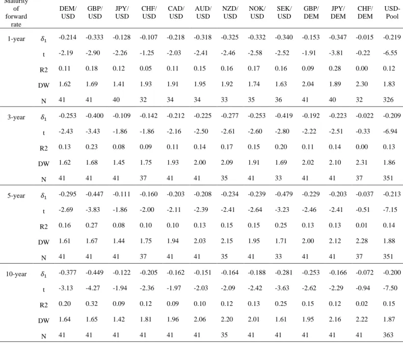
The in-sample one-period slope coefficients from our model are significantly negative when using long-maturity forward rates, as shown in Block 2–4, Panel 1, Table 2. In contrast, when using the one-month maturity forward rate (Block 1, Table 2), slope coefficients tend to be insignificant and smaller in absolute terms, while regressions have lower R². Beyond using monthly data, we also estimated one-period regressions using non-overlapping annual data (see Table A2 in the appendices). The R² associated with annual data for the panel model is 0.15 when using the 10-year forward rate, a rather high value given the spot exchange rate of floating currencies is typically approximated as a random walk. R² are relatively high for all currency pairs except the CHF/DEM rate, with the highest values obtained for the GBP/USD rate (0.32), SEK/USD rate (0.25) and the DEM(EUR)/USD rate (0.20).

4.3. Robust confidence interval for the regression parameter

Theoretical long maturity forward rates are rather persistent time series and might even contain a unit root. The issue of persistent or non-stationary predictors is hardly considered in the exchange-rate forecasting literature¹⁰. For example, this issue is not even mentioned in the literature survey of Rossi (2013) or in the comparative analysis of Cheung et al (2019). We have downloaded the data on predictors used by Cheung et al (2019) and found that the null hypothesis of unit root cannot be rejected for almost 40% the predictors used in their study¹¹.

10 A rare example of testing the time-series properties of the predictor is Engel et al (2007). They could not reject the null hypothesis of no cointegration for one of their three models, implying the error correction term in their forecasting model is non-stationary. However, they still found this unbalanced regression provided superior out- of-sample forecasts.

11 Cheung et al (2019) used eight models of which we could replicate the dataset for six. They considered four US

In our dataset, we found that long maturity theoretical forward rates are stationary for four currency pairs (the US dollar against the German mark, British pound sterling and Canadian dollar, and the rate of the German mark against the British pound sterling), but not for the other six currency pairs¹².

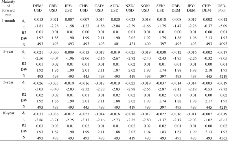
We therefore used the method proposed by Rossi (2007) to calculate confidence intervals of regression parameter of the one-period regression, which method is robust whether the regressor has a unit root or not. Table 3 shows that when the 1-month forward rate is used as the regressor, zero is always within the 95 percent confidence interval. When the 10-year forward rate is used as the regressor, for five of the twelve currency-pairs, zero is not within the confidence interval and for the remaining seven cases, most of the confidence interval range is negative. We therefore conclude that even though theoretical long-maturity forward rates are rather persistent and might even contain a unit root, they can be useful in exchange rate forecasting.

*** Table 3 ***

5. Out-of-sample forecasting 5.1 Forecast evaluation sample

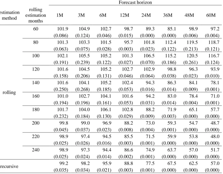
We use the 1979-1989 sample period (or mid-1980s to 1989 when earlier data is not available) to form an initial estimate and evaluate our out-of-sample forecasts for the January 1990 – February 2020 period using forecasting horizons between 1 month and 5 years. We use a recursive estimation scheme¹³ in our baseline forecasting exercise, but as a robustness check

dollar currency pairs (CAD, JPY, CHF and GBP) in their full sample estimations. Of these 6x4=24 cases, we could reject the null hypothesis of unit root (for those predictors for which estimation is not needed) or the null hypothesis of no cointegration (for those models which are based on the estimation of a cointegration relationship) for 15 cases and we could not reject these null hypotheses for 9 cases.

12 Darvas and Schepp (2009) were the first to notice that some long-maturity theoretical forward exchange rates of major currencies are stationary.

also use a rolling estimation scheme with windows of various lengths.

5.2 Statistics

Rossi (2013) highlighted that “The toughest benchmark is the random walk without drift” (p.

1063), which we use as the benchmark for our models. We use four out-of-sample forecasting evaluation criteria.

The first indicator, which is the most widely used in the literature, is the mean squared forecast error (MSFE) relative to the driftless random walk (𝑀𝑆𝐹𝐸𝑅_𝑘):

(14) 𝑀𝑆𝐹𝐸𝑅_𝑘 = 100 ∙ ^{𝑃−1∑(𝑠𝑡+𝑘−𝑠̂𝑀,𝑡,𝑡+𝑘)}

2 𝑃⁻¹∑(𝑠_𝑡+𝑘−𝑠̂_{𝑅𝑊,𝑡,𝑡+𝑘})² ,

where k is the forecast horizon, 𝑠_𝑡+𝑘 is the log exchange rate at period t+k, 𝑠̂_{𝑀,𝑡,𝑡+𝑘} is the log of the forecast made at time t for t+k by our model, 𝑠̂_{𝑅𝑊,𝑡,𝑡+𝑘} is the log of the random walk forecast made at time t for t+k, and P is the number of forecasts made. Therefore, this measure is calculated as a percentage where a value below 100 indicates that our model outperforms the driftless random walk.

The driftless random walk benchmark is nested in all models. When comparing nested models, standard asymptotic tests do not apply when testing the null hypothesis of equal forecast accuracy. Clark and West (2006, 2007) showed that under the null hypothesis that the data generating process is the random walk (or any parsimonious model), estimation of parameters of a larger model introduces noise into the forecasting process that will, in finite samples, inflate its MSFE. Clark and West (2006, 2007) also suggested an adjustment of mean squared prediction error statistics, which leads to approximately normal tests. Clark and West (2006, 2007) derived their results for models estimated in direct form, i.e. in the form of long-horizon regressions, and when the forecasts are evaluated using a rolling-window estimation technique.

1994M12. Next, we estimate the models for 1979M1-1990M1 and calculate out-of-sample forecasts for 1990M2- 1995M1, and so on.

They also found that a bootstrap test has favorable properties in terms of both size and power.

However, Pincheira and West (2016) found that the Clark and West (2006, 2007) statistics also worked reasonably well when the iterated method is used to obtain multi-step forecasts and the recursive estimation scheme is used. For the iterated method they considered a simple first order autoregression for the predictor, in the same way as in our forecasting model (13).

We therefore use two methods to test the null hypothesis of equal MSFE of our model and the random walk against the one-sided alternative that our model is better: (1) a non-parametric bootstrap test similar to those used in related papers such as Mark (1995), Kilian (1999) and McCracken and Sapp (2005), and (2) the Clark and West (2006, 2007) statistics. Since we find that the two methods lead to rather similar results (which we demonstrate for the detailed DEM/USD forecasting results), while calculating bootstrapped p-values is rather time consuming, but the calculation of the Clark and West statistics is instantaneous, in most of this paper we derive the p-values from the Clark and West statistics. For this statistic, we estimate the long-run variance using the method of Newey and West (1987).

The second indicator is the share of correct sign (i.e. direction of change) predictions relative to the spot exchange rate (𝐷𝑂𝐶𝑆_𝑘):

(15) 𝐷𝑂𝐶𝑆_𝑘 = 100 ∙ 𝑃⁻¹∑ 𝐼(𝑠_𝑡+𝑘− 𝑠_𝑡, 𝑠̂_{𝑀,𝑡,𝑡+𝑘}− 𝑠_𝑡),

where the 𝐼(. , . ) is an indicator function having the value 1 if its two arguments have the same sign and zero otherwise. Therefore, this measure is calculated as a percentage where a value above 50 indicates our model predicts the direction of change well more than half of the time.

We use the test developed by Pesaran and Timmermann (1992) to test the null hypothesis that our model has no power in predicting the exchange rate. We use the same test for testing the null hypothesis that the forward exchange rate has no power in predicting the exchange rate.

The third indicator is the share of correct sign (i.e. direction of change) predictions relative to the forward exchange rate (𝐷𝑂𝐶𝐹_𝑘):

(16) 𝐷𝑂𝐶𝐹_𝑘 = 100 ∙ 𝑃⁻¹∑ 𝐼(𝑠_𝑡+𝑘− 𝑓_𝑡, 𝑠̂_{𝑀,𝑡,𝑡+𝑘}− 𝑓_𝑡).

From a currency trading perspective, the share of correct sign predictions relative to the forward exchange rate is more relevant than predicting the direction of change relative to the spot exchange rate, because a forward transaction is settled at the forward rate. The deviation of the future spot rate from the forward rate (and not from the current spot rate) determines whether there is a profit or loss. We are not aware of papers calculating the share of correct sign predictions relative to the forward exchange rate. We again use the test of Pesaran and Timmermann (1992).

The fourth indicator is the excess return on a trading strategy based on our forecasting model where a positive value indicates excess profit. For comparison, we also report the return on a simple carry trade investment strategy.

The carry trade strategy on currency markets postulates that the currency with the higher interest rate is purchased by borrowing in a currency which has a lower interest rate. An equivalent carry trade transaction can be conducted in forward or futures markets, by buying a high-yield currency forward against a low-yield currency. The excess return, ignoring transaction costs and leverage, to the simple carry trade strategy is:

(17) 𝑟_{𝐶𝑇,𝑡+𝑘}^(𝑘) = {

𝑑_𝑡^(𝑘)− 𝑠_𝑡+𝑘 𝑖𝑓 𝑑_𝑡^(𝑘)> 𝑠_𝑡 0 𝑖𝑓 𝑑_𝑡^(𝑘) = 𝑠_𝑡 𝑠_𝑡+𝑘− 𝑑_𝑡^(𝑘) 𝑖𝑓 𝑑_𝑡^(𝑘)< 𝑠_𝑡 .

where 𝑟_{𝐶𝑇,𝑡+𝑘}^(𝑘) is the excess return of the carry trade strategy realized in time t+k for a forward transaction opened in time t for k-period ahead. For example, consider the New Zealand dollar/USD dollar pair over one period. When the New Zealand interest rate is higher than the US interest rate (𝑑_𝑡⁽¹⁾ > 𝑠_𝑡), the New Zealand dollar is purchased against the US dollar and the return in the next period is 𝑑_𝑡⁽¹⁾− 𝑠_𝑡+1. That is, if the New Zealand dollar appreciates (𝑠_𝑡+1 <

𝑠_𝑡), remains unchanged (𝑠_𝑡+1 = 𝑠_𝑡), or depreciates less than the forward premium (𝑠_𝑡+1 <

𝑑_𝑡⁽¹⁾), a profit is realized. This return is in excess of the risk-free rate. To enter a forward or futures transaction, the investor must post a margin in the form of cash or appropriate high- quality marketable securities, such as a government bond. The investor earns interest income from the collateral. Therefore, the payoff for the forward transaction can be regarded as return in excess of the risk-free interest rate, such as a government bond yield. Forward currency market transactions typically involve use of leverage, as only a small percentage of the notional amount of the transaction (for example 4%) is required by the financial intermediator as collateral. However, in our return calculations, we do not consider levered positions or transition costs¹⁴.

The trading strategy return implied by our forecasting model is defined as follows:

(18) 𝑟_{𝑀,𝑡+𝑘}^(𝑘) = {

𝑑_𝑡^(𝑘)− 𝑠_𝑡+𝑘 𝑖𝑓 𝑑_𝑡^(𝑘) > 𝑠_{𝑡+𝑘|𝑡} 0 𝑖𝑓 𝑑_𝑡^(𝑘)= 𝑠_{𝑡+𝑘|𝑡} 𝑠_𝑡+𝑘− 𝑑_𝑡^(𝑘) 𝑖𝑓 𝑑_𝑡^(𝑘) < 𝑠_{𝑡+𝑘|𝑡}

.

where 𝑟_{𝑀,𝑡+𝑘}^(𝑘) is the excess return of an investment strategy based on our model and 𝑠_{𝑡+𝑘|𝑡} is the forecast in period t for period t+k. Continuing the example above, if our forecast suggests the New Zealand dollar will appreciate (𝑠_𝑡+1|𝑡 < 𝑠_𝑡), will remain unchanged (𝑠_𝑡+1|𝑡 = 𝑠_𝑡), or will depreciate less than implied by the forward rate (𝑠_𝑡+1|𝑡 < 𝑑_𝑡⁽¹⁾), the New Zealand dollar is purchased against the US dollar and the return for period t+1 is 𝑑_𝑡⁽¹⁾− 𝑠_𝑡+1.

We report the mean annualized profit over our out-of-sample evaluation period. We test whether the mean annualized profit based on our model is larger than zero and whether it is larger than the profit of carry trade. We test these hypotheses by t-tests based on the Sharpe ratio (profit divided by its standard deviation), for which we estimate the long-run variance using the method of Newey and West (1987).

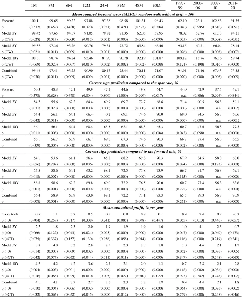
5.3 Baseline results for the German mark / US dollar rate

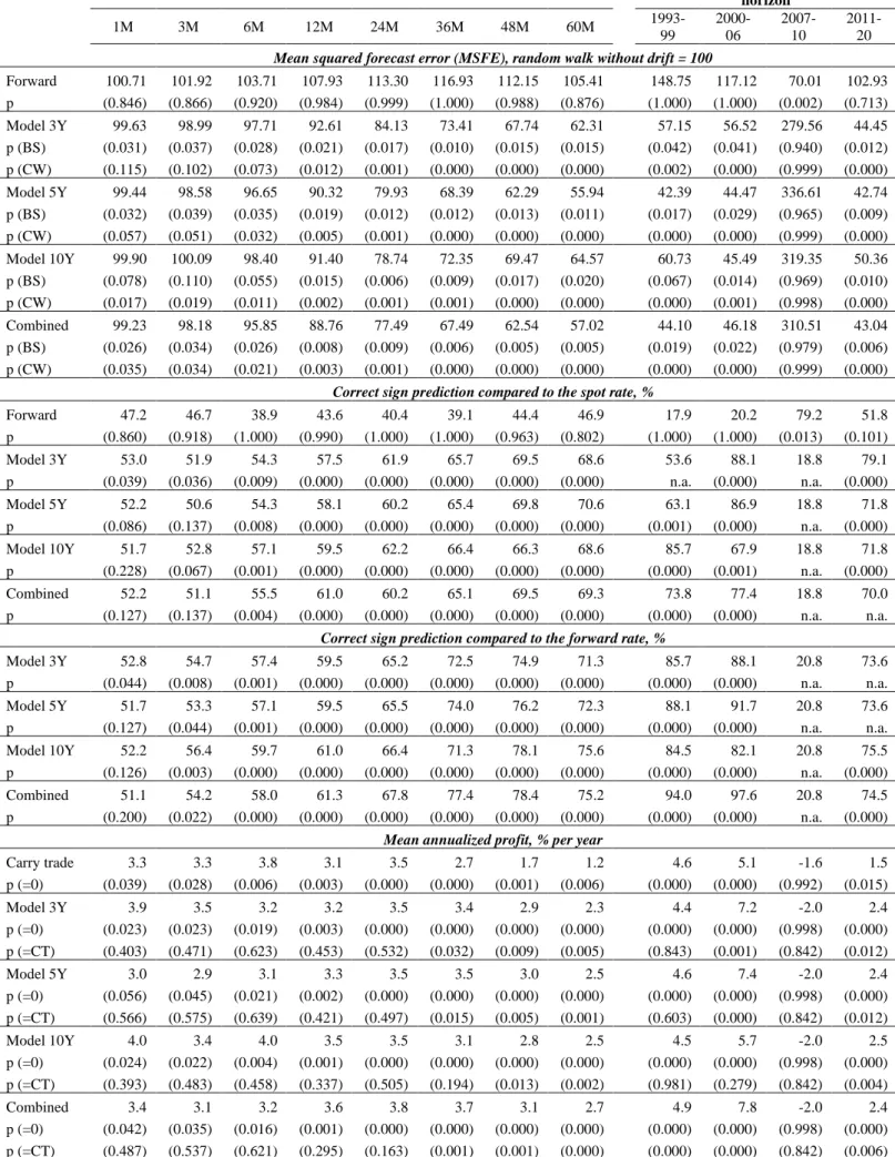
*** Table 4 ***

Table 4 shows baseline results for the USD/DEM exchange rate. Our full-sample results indicate better-than-random walk forecasts for both short and long forecasting horizons, using three alternative maturity forward rates and four forecast evaluation criteria (Table 4). The point estimates of the mean squared forecast error (MSFE) of our models are lower than that of the driftless random walk for forecasting horizons between 1 month and 5 years and for all alternative models using different maturity forward rates, with the sole exception of the model using the 10-year maturity forward rate for 3-month forecasting horizon. In this case the point estimate is also statistically less than 100% at the 11 percent significance level according to our bootstrap test and at 2 percent significance level according to the Clark and West (2006, 2007) test. For all models, longer forecasting horizons are associated with stronger results relative to the driftless random walk. Table 4 also presents results from forecasts using the simple equally- weighted combination of the three models with alternative-maturity forward rates. Our findings corroborate findings from forecast combination literature (see e.g. Timmermann, 2006) showing a simple equal-weight combination performs well. Interestingly, the combined forecast outperforms the best individual model for six of eight alternative forecast horizons reported based on MSFE statistics. The improvement in forecast accuracy as measured by the MSFE of the combined model over the driftless random walk is about 10% for 1-year ahead forecasts, 30% for 3-year ahead forecasts, and about 40% for 5-year ahead forecasts. These are rather large improvements relative to models presented in past works. For example, Rossi (2013) analyzed the predictive ability of six single equation and two multiple-equation models for different sample periods staring between the 1960s and 1990s and ending in mid-2011 and finds the bulk of the MSFE ratios are over 1 (or 100 if expressed it in percent) for both short-horizon

(1 month or 1 quarter) and long horizon (4 years) forecasts. Among the 111 ratios reported for the 4-year forecasting horizon, only two were lower than 1, and both by only 1 percent.

The two alternative ways for testing the null hypothesis that the MSFE of our model is the same as that of the random walk led to rather similar results, in line with the findings of Pincheira and West (2016). The exceptions are few and do not change the big picture.

In contrast to the excellent forecasts of our model, the forward rate itself as a prediction never led to smaller forecast errors than the random walk in our full out-of-sample evaluation period.

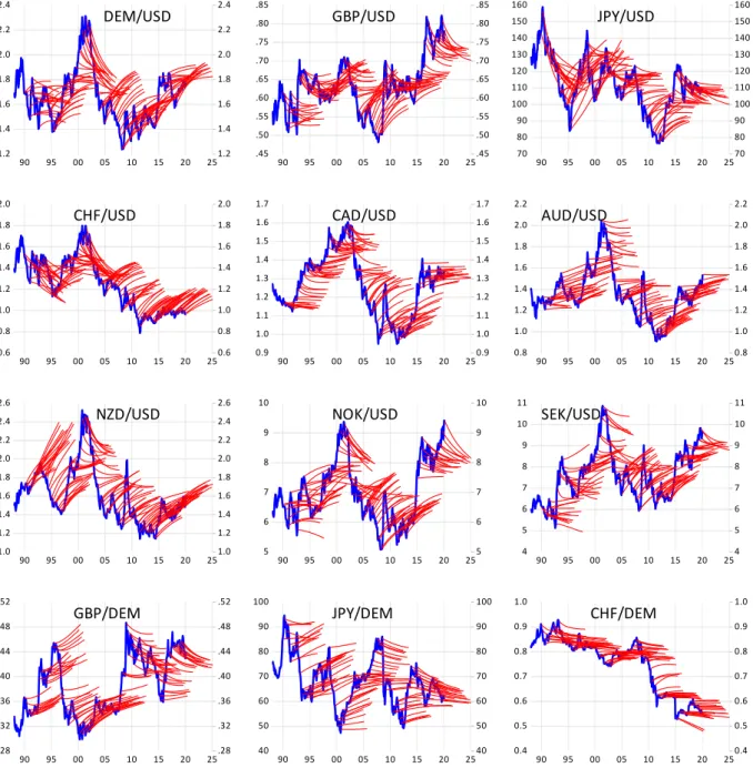
*** Figure 1 ***

The first panel of Figure 1 shows actual exchange rate movements (solid blue line) and out-of- sample forecasts five years ahead (light red lines) using the combined model for the DEM/USD rate. For better readability of the panels, forecasts made only in March, June, September and December of each year are shown. The figure indicates that our model was capable of indicating both upward and downward turning points rather well, although many of the large excessive swings were forecasted to turn around earlier.

Turning to direction of change predictions, our models predict the correct signs in more than half of the cases for all three alternative models, as well as their combination, and for all forecasting horizons between one month and five years. At the one-month horizon correct sign predictions relative to the spot rate were made in about 52-53 percent of cases, while at the five- year horizon in about 70 percent of cases, which is really large. The bulk of these sign predictions are statistically significant. In contrast, the forward rate itself predicts the direction of change in less than 50 percent of cases for all forecast horizons in our full out-of-sample evaluation period.

Correct sign prediction relative to the forward rate is even more impressive, with 75%-78%

correct predictions at 3-5-year horizons by the combined model.

It is therefore not surprising that a trading strategy based on our model leads to profit. The

annualized excess return amounts to about 3 percent per year, which is economically significant, given that the average annualized US dollar interest rate was 3.1% for the one-month interbank rate and 4.5% for the 10-year government bond yield from 1990-2020. The annualized excess returns are significantly larger than zero, though generally not significantly larger than the return based on carry trade on shorter forecasting horizons, but significantly larger on longer forecasting horizons.

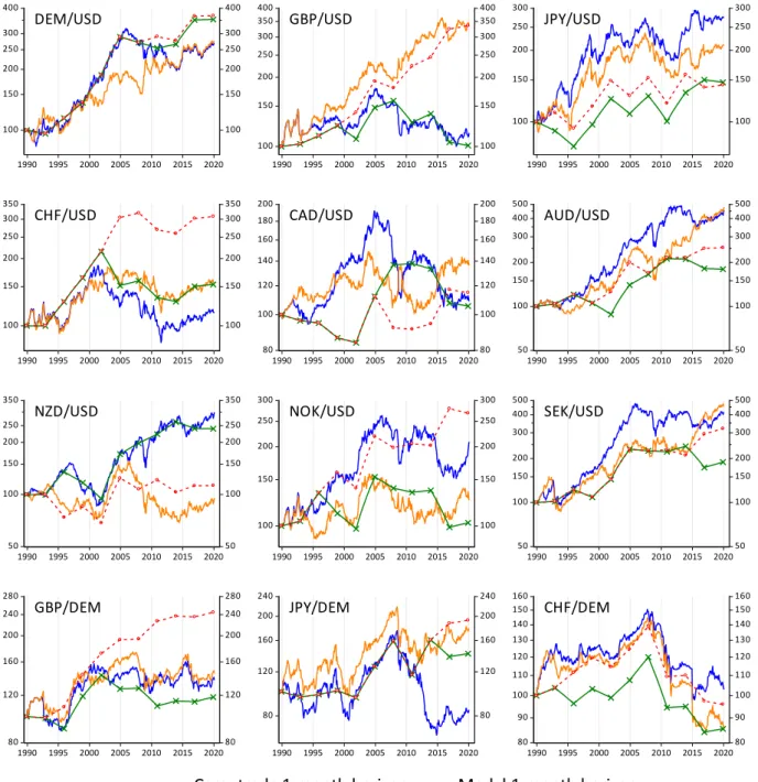
*** Figure 2 ***

By assuming an initial investment value of 100, Figure 2 visualizes the trading profit by considering one-month and three-year reinvestment decisions. That is, in the former case the cumulative value of investment is reinvested according to our one-month ahead forecast for one-month horizon, while for the latter case the investment decision is made in every third year based on our three-year ahead forecasts. The same exercise is made for the carry trade too. For the DEM/USD currency pair, the one-month reinvestment horizon led to rather similar total cumulative returns for our model and the carry trade in 1990-2020, though return volatility is lower in the case of our model than for carry trade returns. For the three-year reinvestment horizon, eight of the ten decisions were the same for our model and for the carry trade. It is therefore not surprising that the overall performance over the 30-year period is rather similar for our model and the carry trade, even though our model led to much lower MSFE than the random walk¹⁵. This finding suggests that better forecasting ability of a model than the random walk might not be associated with significantly better model-based return than the return on carry trade.

15 Note that the 3-year trading simulation reported on Figure 2 is a particular non-overlapping result, showing the cumulative value of an initial investment of 100 made in December 1989. The average annualised 3-year return results reported in Table 4 considers investments made in each month in December 1989 – December 1992, which average is significantly larger in the case of our models than the carry trade returns.

5.4 Other currencies

Because of space constraints and the large number of robustness tests performed, for other currency pairs, we report only the MSFE results based on the combined model. Detailed results for individual models and for all four forecast evaluation criteria are available in the appendices.

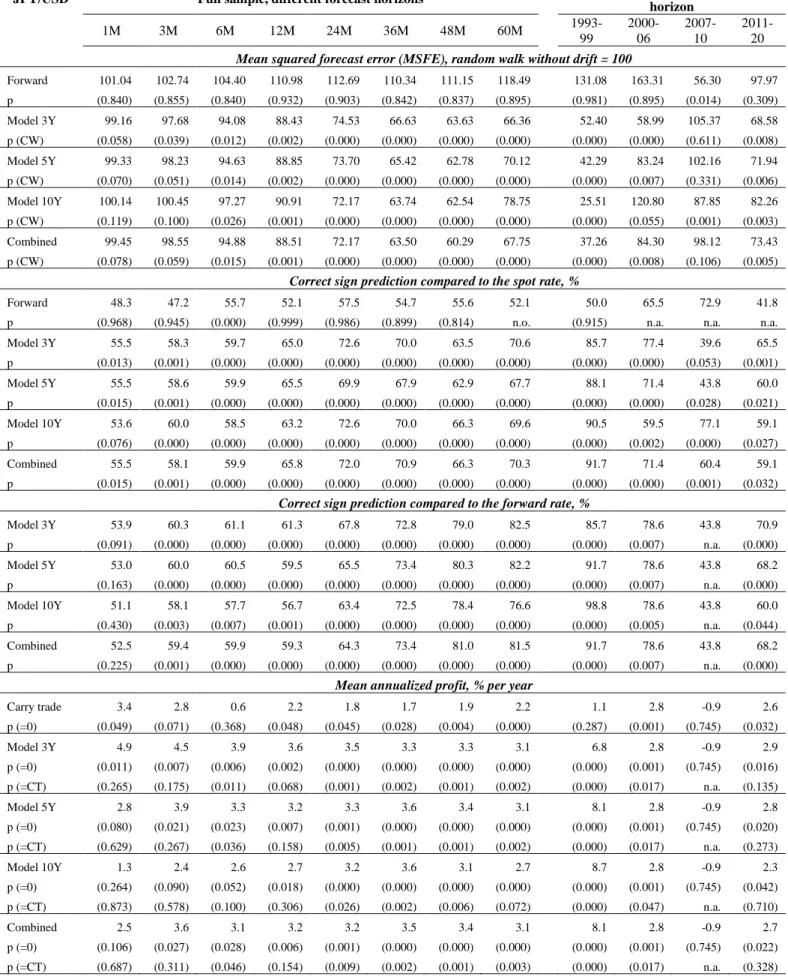
*** Table 5 ***

Our model also performs well for the bulk of the other currency pairs. In particular, both short- and long-horizon forecasts beat the driftless random walk for the US dollar rate relative to the British pound sterling, Norwegian krone, Swedish krona, Australian dollar. The same applies for the Japanese yen when the estimation starts in 1985. Results are also strong for the rate of the German mark relative to the British pound sterling.

For the Canadian dollar-US dollar, New Zealand dollar-US dollar and Japanese yen-German mark/euro pairs, short-term forecasting results are less favorable, while long-term forecasting results beat the random walk. Further research should explore if these somewhat weaker results relate to deviations from the underlying assumptions of the monetary model of exchange rate that we used to derive our forecasting model.

In the case of the Swiss franc/US dollar rate, full sample MSFE statistics are larger than that of the random walk in the baseline specification. However, poor forecasting results over the full sample period are not surprising. As the euro-area crisis escalated after 2010, Switzerland received increasing capital inflows. In September 2011 the Swiss National Bank unexpectedly introduced a floor for the euro/Swiss franc rate at 1.2 to limit currency appreciation. This floor meant effectively fixing the value of the Swiss franc to the euro and remained in place until January 2015. In the sub-sample sensitivity analysis below, we show forecasting results for the Swiss franc/US dollar rate were very strong in the out-of-sample evaluation period from 1990 to 2006. The finding for the rate between the Swiss franc and German mark/euro are similar

and in fact more favorable, since our baseline forecast beats the random walk in our first three sub-periods covering 1990-2010, and the full-sample forecasts are also statistically better than the random walk for forecasting horizons between 1 and 5 years, even if the point estimates are larger than 100. Panel models work even better for the Swiss franc, against both the dollar and the mark/euro.

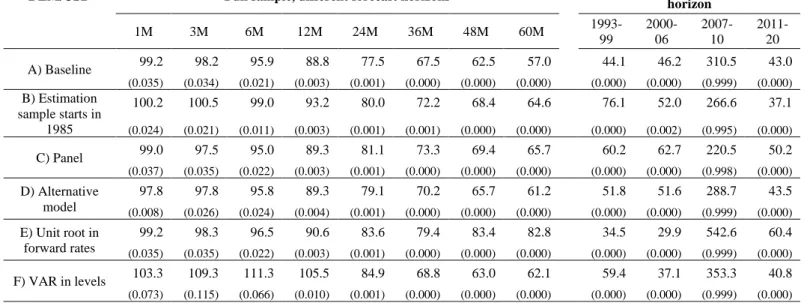
5.5 Sub-sample sensitivity

The last four columns of Table 4 and Table 5 show out-of-sample forecasting results for 3-year ahead predictions using alternative sample periods. For almost all currency pairs, our forecasts beat the random walk in 1993-1999, 2000-2006 and 2011-2020 sub-periods, but not the 2007- 2010 period, which included the global financial and economic crisis. US dollar exchange rate movements during the period were erratic, making forecasting difficult for all models.

Interestingly, our model continues to forecast well in the 2007-2010 period for four currency pairs: British pound sterling relative to the US dollar, British pound sterling relative to the German mark/euro, Japanese yen relative to the German mark/euro, and the Swiss franc relative to the German mark/euro.

Table 4 also indicates stunning sign prediction forecasts in sub-periods which do not include the period of the global financial crisis. For example, the combined model for the German mark/euro rate against the US dollar predicted the deviation from the 3-year forward rate correctly in 94% of the cases in 1993-1999 and 97.6% of the cases in 2000-2006. The 74.5%

correct prediction share in 2011-2020 is also impressive. It is therefore not surprising the model- based trading strategy led to rather high excess returns, amounting to 4.9% per year in 1993- 1999 and 7.8% per year in 2000-2006.

5.6 Dropping 1979-84 data

In our analysis thus far, we have used the 1979-1989 sample period, with a few data driven exceptions, to form an initial estimate and evaluated our forecasts in the 1990-2020 period. The US dollar experienced large price fluctuations in 1980-1984. As a robustness test, we shorten the estimation sample period to start in January 1985, but continue to evaluate the out-of-sample forecasts in 1990-2020.

Table 5 Panel B shows that for most currencies, forecasting results are slightly weaker in this case, though they still beat the random walk by a large margin. Exceptions were the Australian dollar, for which short-term forecast are slightly worse, while long-term forecasts are slightly better than our baseline, and the Japanese yen, for which results are much stronger when the sample starts in 1985¹⁶. The explanation for more favorable Japanese results could be the strong nominal and real appreciation during the 1979-1984 period, while the monetary model assumes purchasing power parity holds in the long run.

Our generally favorable results for the longer sample period may be related to the ability of our model to capture adjustments to the equilibrium value of the exchange rate, which can be better estimated using longer sample periods.

5.7 Panel estimation

Our forecasting exercise thus far has been simple in being based on the analysis of single currency pairs and involving the estimation of only four parameters and with OLS. As a robustness test, we perform panel estimation, where we force parameters 𝜃₂ and 𝜃₄ in model (13) to be common across currency pairs, but allow the intercepts, 𝜃₁ and 𝜃₃, to vary. We find panel estimation improves both short- and long-horizon forecasts in the case of eight currency

16 For the New Zealand dollar and the Swiss franc, results for the sample starting in 1985 are the same as the

pairs (CHF/USD, NOK/USD, SEK/USD, CAD/USD, AUD/USD, NZD/USD, GBP/DEM, JPY/DEM). It is useful to highlight that the full-sample MSFE point estimates are below 100 at all forecasting horizons for the NZD/USD rate and these estimates are statistically

significant. The full-sample results for the CHF/USD rate statistically significantly beat the random walk in all but the 3-month forecasting horizons, though sub-sample results continue to indicate weak forecasts in 2011-2020, which includes the 2011-2015 fixed exchange rate episode. Panel estimation leads to slightly better short-horizon forecasting at the cost of slightly worse long-horizon forecasts for two currency pairs (DEM/USD and GBP/USD).

Panel estimations worsen forecasts considerably for the JPY/USD rate. For the CHF/DEM rate, short-run forecasts are slightly better with panel estimation, but longer-term forecasts are considerably worse. Overall, these results show our findings are robust to single equation versus panel estimation.

5.8 Alternative model

Thus far we have used the simple setup described in model (13). The first equation of this model is an error-correction equation, while the second equation is a simple autoregression for the error-correction term (the theoretical forward rate). An alternative is a standard vector error correction model (VECM):

(19)

𝑠_𝑡+1− 𝑠_𝑡 = 𝜑₁+ 𝜑₂(𝑠_𝑡− 𝑠_𝑡−1) + 𝜑₃(𝑖̃_𝑡^(ℎ)− 𝑖̃_𝑡−1^(ℎ)) + 𝜑₄∙ 𝑑_𝑡^(ℎ)+ 𝜀_𝑡+1,1⁽¹⁾ 𝑖̃_𝑡+1^(ℎ) − 𝑖̃_𝑡^(ℎ) = 𝜑₅+ 𝜑₆(𝑠_𝑡− 𝑠_𝑡−1) + 𝜑₇(𝑖̃_𝑡^(ℎ)− 𝑖̃_𝑡−1^(ℎ)) + 𝜑₈∙ 𝑑_𝑡^(ℎ)+ 𝜀_𝑡+1,1⁽²⁾ , where 𝜑_𝑖 are parameters to be estimated. Model (19) shares the advantageous features of model (13), since it is not estimated in overlapping samples. The model is not subject to the various information losses we described earlier, and multi-step ahead out-of-sample forecasts are calculated with a dynamic iteration method also using the identity defined in equation (10).

Model (19) includes eight parameters to be estimated and can easily be replicated.

As Table 5 Panel D shows, forecasting results using this alternative model are similar to benchmark results and also beat the random walk.

5.9 Unit root in forward rates

From a time series analysis perspective, our models given in equations (13) and (19) correspond to a stationary long-maturity theoretical forward rate assumption. We check the sensitivity of our forecasting results by assuming that the long-maturity forward rate is non-stationary, that is, 𝜃₃ = 0 and 𝜃₄ = 1 in the forecasting model (13), implying the long-maturity forward rate remains unchanged over the forecasting horizon. This assumption influences only multi-period ahead forecasts, but not the 1-month ahead forecasts, because the second equation in model (13) is not used for that.

Forecasting results, presented in Table 5 Panel E, are weaker in this case. For example, in the DEM/USD case at the 5-year ahead forecast horizon, the MSFE ratio is 57.0 in our baseline case, but 82.8 in the unit root case. For the GBP/USD rate at the 5-year ahead forecast horizon the baseline result is 71.1, and 126.4, assuming unit root. Altogether, the unit root assumption worsens forecasting results for eight of our twelve currency pairs, while for the remaining four currency pairs (NOK/USD, AUD/USD, GBP/DEM, JPY/DEM) short-horizon forecasts are almost identical and long-horizon forecasts are slightly better under the unit root

assumption.

5.10 VAR in levels

A vector autoregression model (VAR) in levels can be consistently estimated irrespective of whether the variables have a unit root or not. We therefore employ a simple VAR(1) as a robustness check: