BEAMS UNDER A CENTRAL CONCENTRATED LOAD L´aszl´o Kiss1, Gy¨orgy Szeidl2
1PhD student,2 Professor Emeritus
Institute of Applied Mechanics, University of Miskolc 3515 Miskolc-Egyetemv´aros, Hungary
1. INTRODUCTION
Curved beams have an important role in many engineering structures, e.g. in roof structures and bridges. Research on the mechanical behaviour of these structural elements began in the 19th century – see [1, 1892] and [2, 1906] by Love. The most important results achieved before the sixties of the last century are presented in [3, 1961] by Timoshenko and Gere. Based on a geometrically nonlinear model, analytical solutions for shallow arches subjected to a vertical load at the crown point are provided in [4, 2002] and [5, 2002] by Bradford et al. The former articles are, however, valid only for homogeneous material. In this paper we assume that the radius of curvature is constant and the Young modulus depends on the cross sectional coordinates only. We aim to: (1) derive a model more accurate then those available in the literature, (2) determine the buckling load for a pinned-pinned beam which is subjected to a constant radial dead load at the crown point, (3) compare the results to those obtained by Bradford et al.
2. BASIC ASSUMPTIONS
Figure 1.
Figure 1. shows a portion of the curved beam consid- ered; the orthogonal curvilinear coordinate system(ξηζ) –η =ζ = 0on the (E-weighted) centerline with radius ρo and the unit vectorseξ ,eη andeζ. The cross-section of the beam is symmetric with respect to the axisζ. The point in which the centerline intersects the cross-section is denoted by C. Its position on the cross-section fol- lows from the condition
Qeη = Z
A
E(η, ζ)ζdA = 0 (1) in whichQeη is the E-weighted first moment with respect to the axis η. The Young modulus should satisfy the relationE(η, ζ) =E(−η, ζ). The arc coordinatesis mea- sured from the crown point whileϕ= s/ρois the angle coordinate. The displacement vector at an arbitrary point on the cross-section takes the form
u=uo+ψoηζeξ =woeζ + (uo+ψoηζ)eξ , ψoη = uo/ρo−dwo/ds , (2) where uo = uoeξ +woeζ and ψ = ψoηeη are the displacement and rotation on the centerline. It can be shown that the axial strain is
εξ = (1 +ζ/ρo)−1(εoξ+ζκo) +ψoη2 /2 in which (3a) εoξ = duo
ds +wo
ρo , dψoη
ds =κo =− d ds
dwo ds − uo
ρo
and εm =εoξ+1
2ψoη2 . (3b)
Hereεoξandεmare the linear and nonlinear axial strains on the centerline whileκois the change of curvature. We shall assume thatσξ = E(η, ζ)εξ is the Hooke law. If it is reasonable in the sequel we shall apply the following two notational conventions:
ρnodn(. . .)/dsn = dn(. . .)/dϕn= (. . .)(n), n = 1,2, . . .; m=Aeρ2o/Ieη. (4) Making use of the Hooke law we get the bending moment and the axial force as M =
Z
A
EεξζdA' −Ieη
wo(2)+wo
/ρ2o , N = Z
A
EεξdA 'Aeεm−Ieηκo/ρo; (5) whereAe andIeη are theE-weighted area and the E-weighted moment of inertia:
Ae = Z
A
E(η, ζ)dA , Ieη = Z
A
ζ2E(η, ζ)dA . (6) It can be checked by applying the kinematic equations (3) that
ψoη b= uob/ρo−dwob/ds; εξ b = (1 +ζ/ρo)−1(εoξ b+ζκo b)+ψoηψoη b+ψoη b2 /2;(7) where the subscriptbdenote the increment of the various physical quantities between the pre-buckling and post-buckling state. It can also be shown that
Mb ' −Ieη
w(2)ob +wob
/ρ2o and Nb 'Aeεmb−Mb/ρo . (8) 3. PRE- AND POST-BUCKLING EQUILIBRIUM EQUATIONS
Figure 2. shows the centerline of the beam in the initial configuration (blue line) and in the pre- buckling equilibrium state (red dashed line) as- suming symmetrical support and loading condi- tions. However, the beam has rotationally re- strained pin at the (left) [right] end with a tor- sional spring constant (kγ`)[kγr] –kγ` =kγr = kγ. The loading consists of the distributed forces f = fneζ +fteξ and a concentrated force Pζ(ϕ = 0).
e
e
0
P
f
k kr
Figure 2.
The central angle of the beam is2ϑ. For the pre-buckling state equation
Z
V
σξδεξdV =−Pζδwo|s=0−kγ`ψoηδψoη|−ϑ−kγrψoηδψoη|ϑ+ Z
L
(fnδwo+ftδuo) ds (9)
is the principle of virtual work from where (after some here omitted manipulations) we can get the equilibrium equations, the dynamic boundary conditions and the con- tinuity and discontinuity conditions atϕ = 0if we take into account the arbitrariness of the virtual quantitiesδuo,δwoandδψoη. The equilibrium equations are of the form
dN ds + 1
ρo
dM ds −
N +M ρo
ψoη
+ft= 0, d ds
dM ds −
N +M ρo
ψoη
−N ρo
+fn= 0. (10)
In the sequel we shall focus on that problem for whichfn =ft =kγ`= kγr = 0– i.e., we assume that the pinned-pinned beam is subjected to a constant concentrated force at its crown point. Let us substitute relation (5)2 for the force N into (10)1. What remains is(Aeεm)(1)−(Aeεmψoη)/ρo = 0.Since the productεmψoη is quadratic in the displacements it can be neglected. Therefore we arrive at the equation
ε(1)m = 0 → εm =constant. (11)
Manipulations on (10)2 are not detailed here, only the final form is presented:
Wo(4)+ 2 +χ2−1
Wo(2)+χ2Wo =χ2−1, Wo =wo/ρo, χ2 = 1−mεm. (12) This equation can be compared to that published by Bradford et al. in their series of articles – see, e.g., equation (14) in [4, 2002]. The cited authors have not kept the terms underlined in (12). The effects of our keeping these terms will be evaluated later. The principle of virtual work for the buckled equilibrium state assumes the form
Z
V
σ∗ξδε∗ξdV = −Pζ∗δwo∗|s=0−Pξ∗ δu∗o|s=0− mw¨o∗δw∗o|s=0− m¨u∗oδu∗o|s=0−
− kγ `ψoη∗ δψ∗oη
s(−ϑ) − kγ rψoη∗ δψ∗oη s(ϑ) +
Z
L
(fn∗δw∗o+ft∗δu∗o) ds . (13) Here the asterisk symbol denotes the sum of the change between the initial and the pre-buckling configuration (not remarked specifically) and the increment to the post- buckling equilibrium state (denoted byb) – e.g.ε∗m =εm+εmb. In (13) it is assumed that the stability loss is a dynamical process characterized by a massmplaced where the concentrated force acts. The load can either be a dead one, or a follower one.
Apart from these changes (13) coincides formally with (9). After some manipulations (the details are again neglected) it can be shown that the arbitrariness of the virtual quantities yield the following post-buckling equilibrium equations:
dNb
ds + 1 ρo
dMb
ds − 1 ρo
N +M ρo
ψoη b− 1 ρo
Nb+Mb
ρo
ψoη b+ftb= 0,
d2Mb
ds2 −Nb
ρo
− d ds
N+Nb+M+Mb
ρo
ψoη b+
Nb+Mb
ρo
ψoη
+fnb= 0.
(14)
Assume now – just as in the pre-buckling state – that there is a dead concentrated load only, there is no mass atϕ = 0, and there are no springs at the end points. The structure of equilibrium equation (14)1 is very similar to that of (10)1 except that the last term in (14)1 does not appear in the pre-buckling relation. However, it can be neglected since this product is quadratic in the increments. Therefore repeating the same line of thought resulting in (10)1but now for the increments it follows that
(Aeεmb)(1)−(Aeεmψoηb)/ρo= 0 → ε(1)m b = 0 → εm b= constant. (15) Manipulations on equilibrium equation (14)2 are more complex and are neglected.
The final form is relation (16). Compared to the model of Bradford et al. it is more accurate via the presence of the underlined terms – see equation (39) in [4, 2002].
Wob(4)+(2+χ2−1)Wob(2)+χ2Wob =mεmbh
1−Wo(2)−Woi
, Wob =wob/ρo. (16) 4. SOLUTION FOR THE PRE-BUCKLING STATE
The pre-buckling equilibrium is governed by equations (11) and (12). Due to the sym- metry properties of the supports, the geometry and the loading, the radial displace- ment is an even function of the angle coordinate therefore it is sufficient to consider a half of the beam to tackle the problem – see Figure 3. The general solution satisfying equation (12) is sought on the right half of the beam in the form
Wo = χ2−1
χ2 +A1cosϕ+A2sinϕ− A3
χ2 cosχϕ− A4
χ2 sinχϕ , Ai ∈ R. (17)
The integration constantsAican be determined by utilizing the boundary conditions
e
e
0
P 2
Figure 3.
Table 1.
Pre-buckling boundary conditions Crown point Right end Wo(1)
ϕ=+0 = 0 Wo|ϕ=ϑ= 0 IeηWo(3)
ϕ=+0 = P2ζ Wo(2)
ϕ=ϑ = 0
gathered in Table 1. At the right support the displacement and the bending moment are zero. At the crown point the rotation is zero and there is a jump in the shear force with magnitudePζ/2. Consequently we have the following system of linear equations
0 χ 0 −1
0 0 0 1
cosϑ sinϑ −χ12 cosχϑ −χ12 sinχϑ
−cosϑ −sinϑ cosχϑ sinχϑ
A1 A2 A3 A4
=
0
χ χ2−1
P ϑ
−χ2χ−12 0
. (18)
in whichP = (−Pζρ2oϑ)/(2Ieη) is a dimensionless force. With the normal displace- ment in hand the rotation can also be calculated: ψoη = Uo−Wo(1) ' −Wo(1). Here we have assumed that the tangential displacement has a negligible effect on the rota- tion field due to the shallowness. Since the axial strain is constant on the centerline, we can calculate its value as the mathematical average of this quantity:
εm = 1 ϑ
Z ϑ 0
εm(ϕ)dϕ = 1 ϑ
Z ϑ 0
εoξ+ 1 2ψ2oη
dϕ = I1+I2P ϑ +I3
P ϑ
2
. (19) The integralI1,I2andI3can be expressed in closed forms (details are omitted).
5. SOLUTIONS TO THE POST-BUCKLING STATE
After substituting the solution to the pre-buckling displacement into the right side of equation (16) we get
Wob(4)+ (1 +χ2)Wob(2)+χ2Wob =−mεmb
1−χ2 χ2
1
1−χ2 +A3cosχϕ+A4sinχϕ
. (20)
Given thatεmb is constant, it can be averaged as εmb ' 1
2ϑ Z ϑ
−ϑ
Uob(1)+Wob+ψoη bψoη
dϕ = 1 2ϑ
Z ϑ
−ϑ
Uob(1)+Wob+
Uob−Wob(1)
Uo−Wo(1)
dϕ ≈ 1 2ϑ
Z ϑ
−ϑ
Uob(1)+Wob+Wob(1)Wo(1)
dϕ. (21) Observe that ψoη ≈ −Wo(1) is an odd function of ϕ, consequently if Wob is an odd function ofϕ then the above integral vanishes: εmb = 0. Otherwise – practically if Wobis an even function inϕ–εmb is constant. These observations are naturally valid for homogeneous beams as well [5, 2002]. Consequently, ifεmb = constant 6= 0we have to solve equation (20) and ifεmb = 0we get the homogeneous DE
Wob(4)+ (1 +χ2)Wob(2)+χ2Wob = 0 (22)
which follows from (20). It is also important to mention that after buckling every physical quantity is continuous through the intervalϕ ∈ [−ϑ;ϑ] because there is no increment in the loading. The general solution of equation (20) takes the form
Wob=C1cosϕ+C2sinϕ+C3sinχϕ+C4cosχϕ−mεm b
2χ3 2
χ +A3ϕsinχϕ−A4ϕcosχϕ
(23)
withCi∈ R, while the displacement satisfying relation (22) is sought in the form Wob(ϕ) =E1cosϕ+E2sinϕ+E3sinχϕ+E4cosχϕ; Ei ∈R . (24) HereCiandEi are undetermined integration constants.
As mentioned we can talk about symmetric (or limit point) buckling and antisymmet- ric (or bifurcation) buckling. If the buckled shape is [antisymmetric](symmetric) then [εmb = 0] (εmb 6= 0). These possibilities are shown on the [left](right) side in Figure 4. The blue line represents the centerline of the beam in the initial configuration, the red line is the pre-buckling shape, while the green line is the buckled shape.
0
0
P
P
Figure 4.
First let us deal with the simpler antisymmetric buckling. As all fields are continu- ous we now consider the whole beam, consequently the displacement and the bending moment are zero at the end points. After substituting solution (24) into the boundary conditions (BCs) in Table 2, we arrive at a homogeneous system of linear equations for which nontrivial solution exists if the determinant of the coefficient matrix is zero:
D= (1−χ)2(1 +χ)2 sinχϑ cosχϑ cosϑ sinϑ= 0. (25) Recalling the relation χ2 = 1− mεm; we can come to the conclusion that there is only one physically possible solution that issinχϑ= 0 →χ =π/ϑthus
εm = 1
m 1−χ2
= 1 m
1−π ϑ
2
(26) is the lowest (critical) strain. If we now substitute this solution back to the equation system we can check that E1 = E2 = E4 = 0. Consequently it follows from the general solution (24) that the shape of the beam is antisymmetric whenεmb = 0since
Wob(ϕ) =E3sinπ
ϑϕ. (27)
Table 2.
Post-buckling BCs Left end Right end Wob|ϕ=−ϑ= 0 Wob|ϕ=ϑ= 0 Wob(2)
ϕ=−ϑ= 0 Wob(2)
ϕ=ϑ= 0
Table 3.
Post-buckling BCs (symmetric shape) Crown point Right end Wob(1)
ϕ=0= 0 Wob|ϕ=ϑ = 0 Wob(3)
ϕ=0= 0 Wob(2)
ϕ=ϑ= 0
When solving equation (20) it is sufficient to consider the right half of the beam.
The boundary conditions are presented in Table 3. Upon substitution of solution (23) into the boundary conditions we arrive at an inhomogeneous system of equations:
0 −2χ3 −2χ4 0
0 −2χ −2χ4 0
cosϑ sinϑ sinχϑ cosχϑ 2χ2cosϑ 2χ2sinϑ 2χ4sinχϑ 2χ4cosχϑ
C1
C2
C3
C4
=
=mεmb
A4
3A4 1
2χ3
2
χ+A3ϑsinχϑ−A4ϑcosχϑ
A3(χϑsinχϑ−2 cosχϑ)−A4(2 sinχϑ+ϑχcosχϑ)
(28) which can be solved in a closed form. The solutions are, however, not detailed. With Wob; the rotation increment isψoη b' −Wob(1)if we neglect the effect of the tangential displacement on the angle of rotation. Now equation (21) can be rewritten as
εmb ' 1 ϑ
Z ϑ 0
Wob+Wo(1)Wob(1)
dϕ. (29)
If we now substitute all the previously determined kinematical quantities into the above equation, perform the integration and simplify by the incrementεmb; we get
1 =J1+J2P ϑ +J3
P ϑ
2
→ Jˆ1+J2P ϑ +J3
P ϑ
2
= 0, Ji ∈ R. (30) Here each of the integralsJi can be expressed in a closed form.
6. COMPUTATIONAL RESULTS
We compare the outcomes of our model to that derived in [5, 2002] by Bradford et al. Since the present model keeps some terms the cited authors have neglected; we expect improved results regarding the critical load. The achievements of [5, 2002] – in a comparison with finite element calculations – seem to fit well as long asϑ < π/4.
However, we are evaluating the cited model for greater central angles as well to make the differences more spectacular. To facilitate the evaluation process – following the footsteps of Bradford et al. – we introduce a modified slenderness ratio: λ=√
mϑ2. Altogether we can distinguish four different intervals regarding the stability. The limit of each one is a function of the parametermas λ = λ(m). These intervals are collected in Table 4. If we compare these results to that of Bradford et al. (whose limits do not depend on m and are λ = 3.91;λ = 7.96 and λ = 9.8 in the same order as in the table) slight differences can be observed which become greater asm decreases. It is also clear that the antisymmetric shape (bifurcation) dominates.
Table 4.
m
1 000 10 000 100 000 1 000 000
λ <3.80 λ <3.87 λ <3.89 λ <3.90 no buckling
3.80< λ <7.90 3.87< λ <7.95 3.89< λ <7.97 3.90< λ <7.97 limit point only 7.90< λ <9.67 7.95< λ <10.05 7.97< λ <10.18 7.97< λ <10.22 bifurcation point after limit point
λ >9.67 λ >10.05 λ >10.18 λ >10.22 bifurcation point before limit point
Antisymmetric (or bifurcation) buckling occurs when the strain reaches the lowest critical strain which is obtained from the conditionχϑ = π. Substituting it into the
pre-buckling equilibrium equation (19), we can calculate the critical dimensionless load in terms of the geometry – see Figure 5.
Figure 5.
For any fixedm, if ϑis small the two models yield very similar results and the limit values for the two models are not functions ofm. The maximum difference from each other is at most ≈ 4.7% if ϑ = π/4 and it is ≈ 14% if ϑ = 1.4. What is of more importance, the new model yields quite the same or lower buckling loads. Bradford et al. have also published a formula for whenϑ > π/4– see [5, 2002]. It is presented in Figure 5. but it is unclear under what assumptions they have achieved it.
Symmetric (or limit point) buckling can only occur when εmb 6= 0. To tackle this problem we have equations (19) and (30) to be solved together so that we can get the the critical strain and the critical load. Results between the lower and upper limits of the interval in which symmetric buckling shape governs, are shown in Figure 6. Ifm is sufficiently great there is hardly any noticeable difference between the two models (except the limits). However, if m = 1 000 the maximum difference is up to 10%.
Interestingly, this time the new model always predicts greater critical loads.
Figure 6.
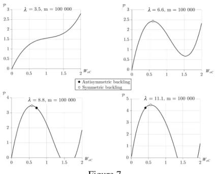
Choosing m = 100 000 we have drawn the primary equilibrium paths for four values ofλ. The reason is that there belongs a different path type to each geometry. In
Figure 7 the dimensionless concentrated forceP is plotted against the dimensionless vertical displacementWoC =Wo(ϕ= 0)/(1−cosϑ)at the crown point.
Figure 7.
Ifλ = 3.5the slope is always positive – there is no buckling. Whenλ = 6.6there is a limit point, i.e. symmetric buckling occurs. Ifλ = 8.8, a bifurcation point appears, but after the limit point, so still the symmetric shape dominates. Whenλ = 11.1the bifurcation point is before the limit so we can expect an antisymmetric buckled shape.
7. CONCLUDING REMARKS
For pinned-pinned curved beams with cross-sectional inhomogeneity we have set up and evaluated a model for in-plane stability investigations provided that the beam is subjected to a radial force at the crown point. We remark that our relations are more accurate than equations (14) and (39) solved by Bradford et al. in [4, 2002], [5, 2002].
Comparing the two models we can come to the conclusions that (a) the stability limits are slightly different, (b) the new model allows at most ≈ 14% lower loads for antisymmetric buckling and (c) ≈ 10% greater loads for symmetric buckling.
Differences are greater ifmis smaller and ifϑis greater.
Acknowledgements by the first author: This research was supported by theEuro- pean Unionand theState of Hungary, co-financed by the European Social Fund in the framework of T ´AMOP-4.2.4.A/2-11/1-2012-0001 ’National Excellence Pro- gram’.
REFERENCES
[1] A. E. H. Love.A treatise on the mathematical theory of elasticity I. and II.Cambridge University Press, 1892 and 1893.
[2] A. E. H. Love.A treatise on the mathematical theory of elasticity. Cambridge University Press, Second edition, 1906.
[3] S. P. Thimosenko and Gere.Theory of Elastic Stability. Engineering Sociaties Monograps. McGraw-Hill, 2ndedition, 1961.
[4] Y. L. Pi, M. A. Bradford, and B. Uy. In-plane stability of arches.International Journal of Solids and Structures, 39:105–125, 2002.
[5] B. Uy M. A. Bradford and Y-L. Pi. In-plane elastic stability of arches under a central concentrated load.
Journal of Engineering Mechanics, 128(7):710–719, 2002.