Vibrations of heterogeneous curved beams subjected to a radial force at the crown point

5th International Conference

on "Computational Mechanics and Virtual Engineering"

COMEC 2013

24 - 25 OCTOBER 2013, Bra¸sov, Romania

VIBRATIONS OF HETEROGENEOUS CURVED BEAMS SUBJECTED TO A RADIAL FORCE AT THE CROWN POINT

György Szeidl¹,László Kiss¹

1Department of Mechanics, University of Miskolc, Miskolc, HUNGARY gyorgy.szeidl@uni-miskolc.hu, mechkiss@uni-miskolc.hu

Abstract: This paper is concerned with the vibrations of heterogenous curved beams under the assumption that the load on the beam is perpendicular to the centerline. It is assumed that (a) the radius of curvature is constant and (b) the Young modulus and Poisson number depend on the cross sectional coordinates only. We have the following objectives: (1) to determine the Green function matrices for pinned beams, fixed beams and beams fixed at one end and pinned at the other end provided that the beam is subjected to a radial load; (2) to clarify how the load affects the natural frequencies if the beam is subjected to a radial force (a vertical force) at the crown point; (3) to develop such a numerical model which makes possible to determine how the natural frequencies are related to the load.

We shall present the computational results in a graphical format.

Keywords:curved beams, heterogeneous material, natural frequency as a function of the load, Green function matrices 1. INTRODUCTION

Curved beams are used in various practical applications. We can mention, for example, arch bridges, roof structures, and stiffeners in aerospace applications. We remark that research into the mechanical behavior of curved beams began in the 19^thcentury – see book [1, 1944] by Love for further details. The free vibrations of curved beams have been extensively investigated. Survey papers on the vibrations of these beams were published by Markus and Nanasi [2, 1981], Laura and Maurizi [3, 1987] as well as Chidampram and Lessia [4, 1993]. It may be worth citing the PhD thesis by Szeidl [5, 1975]

which clarifies within the framework of the linear theory how the extensibility of the centerline affects the free vibrations and stability of circular beams subjected to a constant radial load (dead load). Solutions for the natural frequencies in [5, 1975] were computed by utilizing different numerical models. One of them is based on the use of the Green function matrix of the corresponding boundary value problem. Unfortunately the results of this work have not been published in English.

Paper by [6, 2005] Lawther attacks the problem how a prestressed state of the body affects the natural frequencies.

He studies finite dimensional multiparameter eigenvalue problems and comes to the conclusion that for multiparameter problems, the eigenvalue part of the solution is described by interaction curves in an eigenvalue space, and every such eigenvalue solution has an associated eigenvector. If all points on a curve have the same eigenvector then the curve is necessarily a straight line, but the converse is far more complex.

In the light of Lawther’s results there arises the question how the natural frequencies change if a curved beam is subjected to a radial (vertical) load at the crown point. During our investigations we shall assume that the curved beam is made of heterogenous, isotropic and linearly elastic material. As regards heterogeneity it is assumed that the elastic parameters can be varied arbitrarily over the beam cross section but they are independent of the coordinate perpendicular to the cross section. Under these assumptions our main objectives are as follows: (1) derivation of those boundary value problems which make it possible to clarify how the radial load affects the natural frequencies of the beam; (2) determination of the Green function matrices that can be used to reduce the eigenvalue problems set up for the natural frequencies (which depend on the load) to eigenvalue problems governed by systems of Fredholm integral equations; (3) to reduce the eigenvalue problem to an algebraic one which can be solved numerically. The corresponding computational results are then presented in a graphical format.

The paper is organized into eight sections. Section 2 is a summary of the governing equations. After having defined the Green function matrices we reduced the eigenvalue problems to be solved to eigenvalue problems governed by Fredholm integral equations in Section 3. As regards the solution algorithm Section 4 provides an outline. Calculation of the Green function matrices is detailed in Section 5. Relationships between the axial strain on the centerline and the load are presented in Section 6 which also contains formulae for the critical value of the axial strain. Computational result are shown in Section 7. The last section is a conclusion.

2. GENERALIZATIONS OF SOME CLASSICAL FORMULAE

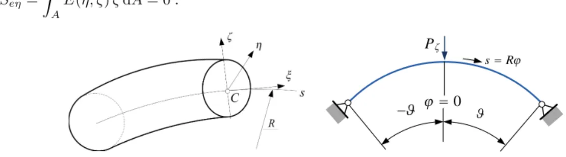
On the basis of article [7, 2012] the most important formulae are all gathered in this section. Figure 1. shows a part of the beam with the applied curvilinear coordinate system (ξ=s, η, ζ) and a pinned-pinned beam. Observe that the coordinate lineξ=scoincides with the so-called (E-weighted) centerline. PointCdetermines the location of the centerline uniquely via equation

Seη= Z

A

E(η, ζ)ζdA= 0. (1)

  0 

sR

P_

Figure 1. (a) The coordinate system, (b) Pinned-pinned beam

HereSeηis the E-weighted first moment of the cross section with respect to the axisη. By assumption the cross section of the beam is symmetric with respect to the axisζand the Young modulus depends on the cross sectional coordinates only:E(η, ζ) =E(−η, ζ).

For our latter considerations let us introduce the integrals Ae=

Z

A

E(η, ζ)dA , Ieη= Z

A

E(η, ζ)ζ²dA (2)

which are referred to as theE-weighted area and theE-weighted moment of inertia.

In what follows we shall separate the load-induced, and otherwise time-independent, mechanical quantities from those which belong to the vibrations of the loaded beam. The latter ones are actually the time-dependent increments and are uniformly denoted by a subscriptb. Letuo,woandRbe the tangential and radial displacements and the radius of the centerline, respectively. The connection between the coordinate linesand the angle coordinateϕis defined bys=Rϕ.

The axial strainε_oξand the rotationψ_oηon the centerline can be given in terms ofu_oandw_oas εoξ =duo

ds +wo

R, ψoη =uo

R −dwo

ds . (3)

On the basis of the principle of virtual work, after some here omitted manipulations, we obtain that the axial forceNand the bending momentM should satisfy equilibrium equations

dN ds + 1

R dM

ds −

N+M R

ψoη

+ft= 0, (4a)

d ds

dM ds −

N+M

R

ψoη

−N

R +fn= 0 (4b)

where the intensity of the distributed loads on the centerline in the tangential and normal directions are denoted byftand fn, respectively.

The axial forceN and the bending momentM are related to the deformations via the Hook law:

N = Ieη

R²εoξ−M

R , M =−Ieη

d²wo

ds² + wo

R²

, N+M R = Ieη

R²εoξ, where m= AeR² Ieη

−1. (5) For our later considerations we introduce dimensionless displacements and a notational convention for the derivatives:

Uo= uo

R , Wo=wo

R ; (. . .)⁽ⁿ⁾= dⁿ(. . .)

dϕⁿ , n= 0,1,2, . . . . (6)

Upon substitution of the Hooke law (5) and then the kinematical quantities (3) into equilibrium equations (4) we arrive at a system of differential equations:

0 0 0 1

U_o W_o

(4)

+

−m 0 0 2−mε_oξ

U_o W_o

(2)

+

+

0 −m

m 0

Uo

Wo

⁽¹⁾ +

0 0 0 1 +m(1−εoξ)

Uo

Wo

= R³ Ieη

ft

fn

. (7)

As regards the increments in the axial strain and in the rotation the corresponding formulae have a structure similar to that of equations (3):

εmb=εoξ b+ψoηψoη b, ψoη b= uob

R −dwob

ds , εoξ b=duob

ds +wob

R . (8)

Further it can be verified that the differential equations the increments in the axial force and in the bending moment should satisfy assume the forms

d ds

N_b+Mb

R

− 1 R

N+M

R

ψ_{oη b}+f_tb= 0, (9a)

d²Mb

ds² −Nb

R − d ds

N+M

R

ψoη b+

Nb+Mb

R

ψoη

+fnb= 0. (9b)

Since the process is a dynamical one – there are no changes in the original loads – it follows that the incrementsf_tband f_nbare in fact forces of inertia, that is,

f_tb=−ρaA∂²u_ob

∂t² , f_nb=−ρaA∂²w_ob

∂t² . (10)

HereAis the area andρais the averaged density over the cross section. In addition the Hooke law for the increments in the inner forces yields

Nb =I_eη

R²mεoξ b−M_b

R , Mb=−Ieη

d²w_ob ds² +w_ob

R²

, Nb+M_b R = I_eη

R²mεoξ b. (11a)

A comparison of equations (8), (9) and (11) results in the equations of motion 0 0

0 1

U_ob W_ob

(4)

+

−m 0 0 2−mε_oξ

U_ob W_ob

(2)

+

+

0 −m

m 0

U_ob W_ob

(1)

+

0 0 0 1 +m(1−ε_oξ)

U_ob W_ob

= R³ Ieη

f_tb f_nb

. (12) Observe that during the formal derivations we linearized the problem: (a) we neglected the quadratic termε_oξε_{oξ b}in (9a);

(b) we took the inequalitiesε_{oξ b}(ε_{oξ b}ψ_oη)⁽¹⁾and1ε_oξinto account in (9b) when we utilized the Hooke law.

If we assume harmonic vibrations and denote the dimensionless displacement amplitudes byUˆ_ob andWˆ_ob then we have

0 0 0 1

Uˆ_ob Wˆob

⁽⁴⁾ +

−m 0 0 2−mε_oξ

Uˆ_ob Wˆob

⁽²⁾ +

+

0 −m

m 0

Uˆ_ob Wˆob

⁽¹⁾ +

0 0 0 1 +m(1−ε_oξ)

Uˆ_ob Wˆob

=λ Uˆ_ob

Wˆob

; λ=ρaAR³ Ieη

α² (13) whereλis the eigenvalue sought andαis the natural frequency of the arch.

For an unloaded beam – i.e. whenεoξ = 0– we get back the equations which govern the free vibrations – compare equation

0 0 0 1

Uˆob

Wˆ_ob ⁽⁴⁾

+

−m 0

0 2

Uˆob

Wˆ_ob ⁽²⁾

+

0 −m

m 0

Uˆob

Wˆ_ob ⁽¹⁾

+

+

0 0 0 m+ 1

Uˆob

Wˆ_ob

=λ Uˆob

Wˆ_ob

(14) to equation (11) in [8, 2013]. Depending on the supports applied the above system should be associated with appropriate boundary conditions. The left side of equation (13) can be rewritten in the form

K[y(ϕ), εoξ] =

4

Py⁽⁴⁾+

2

Py⁽²⁾+

1

Py⁽¹⁾+

0

Py⁽⁰⁾, y= Uˆ_ob

Wˆob

. (15)

It is easy to see that the operatorKis self-adjoint.

Differential equations (14) (or which is the same equations (15)) and the boundary conditions valid for pinned-pinned beams, fixed-fixed beams and beams pinned at one end and fixed at the other end constitute three eigenvalue problems.

Observe that thei-th eigenfrequencyα_i in these eigenvalue problems depend on the magnitude of the concentrated forceP_ζ, or what is the same, on the dimensionless loadP =P_ζR²ϑ/(2I_eη)through the axial strain:ε_oξ=ε_oξ(P). We also remark that the heterogeneity appears in the formulation via the parametersmandρ_a.

3. THE GREEN FUNCTION MATRIX

Observe that differential equations (15) are degenerated since the matrix

4

Phas no inverse. Letr(ϕ)be a prescribed inhomogeneity. Consider the boundary value problems defined by

K(y) =

4

X

ν=0 ν

P(ϕ)y^(ν)(ϕ) =r(ϕ),

3

P(ϕ) = 0 (16)

and the boundary conditions valid for pinned beams:

Uˆ_ob(−ϑ) = 0 Wˆ_ob(−ϑ) = 0 Wˆ_ob⁽²⁾(−ϑ) = 0 | Uˆ_ob(ϑ) = 0 Wˆ_ob(ϑ) = 0 Wˆ_ob⁽²⁾(ϑ) = 0, (17a) for fixed beams:

Uˆ_ob(−ϑ) = 0 Wˆ_ob(−ϑ) = 0 Wˆ_ob⁽¹⁾(−ϑ) = 0 | Uˆ_ob(ϑ) = 0 Wˆ_ob(ϑ) = 0 Wˆ_ob⁽¹⁾(ϑ) = 0, (17b) and for beams fixed at the left end and pinned at the right end:

Uˆ_ob(−ϑ) = 0 Wˆ_ob(−ϑ) = 0 Wˆ_ob⁽¹⁾(−ϑ) = 0 | Uˆ_ob(ϑ) = 0 Wˆ_ob(ϑ) = 0 Wˆ_ob⁽²⁾(ϑ) = 0. (17c) General solution for the homogenous part of differential equations (16) assumes the form

y=

" ₄ X

i=1

Y

(2×2)i C

(2×2)i

# e

(2×1) (18a)

where Y₁=

cosϕ 0 sinϕ 0

, Y₂=

−sinϕ 0 cosϕ 0

, Y₃=

cosχϕ Mϕ χsinχϕ −1

, Y₄=

−sinχϕ 1 χcosχϕ 0

. (18b) HereC_iis an arbitrary constant matrix,eis an arbitrary column matrix and

M= m+ 1

m(1 +εoξ). (18c)

Solutions to the boundary value problems (16,17a), (16,17b) and (16,17c) are sought in the form y(ϕ) =

Z b a

G(ϕ, ψ)r(ψ)dψ , G(ϕ, ψ) =

G₁₁(ϕ, ψ) G₁₂(ϕ, ψ) G₂₁(ϕ, ψ) G₂₂(ϕ, ψ)

(19) whereG(ϕ, ψ)is the Green function matrix defined by the following properties [5, 1975]:

(1) the Green function matrix is a continuous function ofϕ andψ in each of the triangles−ϑ ≤ ϕ ≤ ψ ≤ ϑand

−ϑ≤ξ≤ϕ≤ϑ. The functions(G₁₁(ϕ, ψ), G₁₂(ϕ, ψ)) [G₂₁(ϕ, ψ), G₂₂(ϕ, ψ)]are (2times) [4times] differentiable with respect toϕand the derivatives

∂^νG(ϕ, ψ)

∂x^ν =G^(ν)(ϕ, ψ) (ν = 1,2), ∂^νG2i(ϕ, ψ)

∂x^ν =G^(ν)_2i (ϕ, ψ) (ν= 1, . . . ,4; i= 1,2) are continuous functions ofϕandψ.

(2) Letψbe fixed in[−ϑ, ϑ]. Though the function and the derivatives

G11(ϕ, ψ), G⁽¹⁾₁₂(ϕ, ψ), G^(ν)₂₁(ϕ, ψ) (ν= 1,2,3), G^(ν)₂₂(ϕ, ψ) (ν = 1,2) (20) are continuous everywhere the derivativesG⁽¹⁾₁₁(ϕ, ψ)andG⁽³⁾₂₂(ϕ, ψ)have a jump ifϕ=ψ:

ε→0lim

hG⁽¹⁾₁₁(ϕ+ε, ϕ)−G⁽¹⁾₁₁(ϕ−ε, ϕ)i

= 1/

1

P₁₁(ϕ), , lim

ε→0

hG⁽³⁾₂₂(ϕ+ε, ϕ)−G⁽³⁾₂₂(ϕ−ε, ϕ)i

= 1/

4

P₂₂(ϕ). (21) (3) Letαbe an arbitrary, otherwise constant vector. For a fixedϕ ∈ [−ϑ, ϑ]the vectorG(ϕ, ψ)αas a function ofϕ (ϕ6=ψ) should satisfy the homogeneous differential equationK[G(ϕ, ψ)α] = 0.

(4) The vectorG(ϕ, ψ)αas a function ofϕshould satisfy the boundary conditions (17a), (17b) and (17c) – there belongs one Green function matrix to each of the boundary value problems considered.

If the Green function matrix – defined above for the boundary value problems considered – exists, then vector (19) satisfies differential equation (16) and boundary conditions (17).

Consider the system of differential equations

K[y] =λy (22)

whereK[y]is given by (16) andλis a parameter (the eigenvalue sought). The system of ordinary differential equations (16) is associated with linear homogeneous boundary conditions (17) – they together constitute three eigenvalue problems.

The vectorsu^T = [u1|u2]andv^T = [v1|v2]are said to be comparison vectors if they are different from zero, satisfy the boundary conditions and are differentiable as many times as required.

The eigenvalue problems (16), (17) are self adjoint if the product (u,v)_M = Rϑ

−ϑu^TKvdϕ is commutative, i.e., (u,v)M = (v,u)M over the set of comparison vectors and it is positive definite if (u,u)M > 0for any comparison vectoru.

If the eigenvalue problems (16), (17) are self adjoint then the Green function matrices are cross symmetric:G(ϕ, ψ) = G^T(ϕ, ψ).

4. NUMERICAL SOLUTION TO THE EIGENVALUE PROBLEMS

With (19) the eigenvalue problems (16), (17) can be replaced by homogeneous integral equation systems of the form y(ϕ) =λ

Z ϑ

−ϑ

G(ϕ, ψ)y(ψ)dψ . (23)

Numerical solution to any eigenvalue problem determined by (23) can be sought by quadrature methods [9, 1977]. Con- sider the integral formula

J(φ) = Z ϑ

−ϑ

φ(ψ) dψ≡

n

X

j=0

wjφ(ψj) ψj∈[−ϑ, ϑ] (24)

whereψj(ϕ)is a vector and the weightswjare known. Making use of the latter equation we obtain from (23) that

n

X

j=0

w_jG(ϕ, ψ_j)˜y(ψ_j) = ˜κ˜y(ϕ) κ˜= 1/˜λ ∈[−ϑ, ϑ] (25) is the solution which yields an approximate eigenvalue˜λ= 1/˜κand a corresponding approximate eigenfunctiony(ϕ).˜ After settingϕtoψi(i= 0,1,2, . . . , n)we have

n

X

j=0

w_jG(ψ_i, ψ_j)˜y(ψ_j) = ˜κ˜y(ψ_i) κ˜= 1/λ˜ ψ_i, ψ_j ∈[−ϑ, ϑ] (26) or

GDY˜= ˜κY˜ (27)

whereG= [G(ψi, ψj)]is symmetric if the problem is self adjoint, D= diag(w0, . . . , w0

| {z }

l

|. . .|wn, . . . , wn

| {z }

l

)

andY˜^T = [˜y^T(ψ0)|˜y^T(ψ1)|. . .|˜y^T(ψn)]. After solving the generalized algebraic eigenvalue problem (27) we have the approximate eigenvalues˜λrand eigenvectorsYrwhile the corresponding eigenfunction is obtained by a substitution into (25):

y˜r(ϕ) = ˜λr n

X

j=0

wjG(ϕ, ψj)˜yr(ψj) r= 0,1,2, . . . , n . (28) Divide the interval[−ϑ, ϑ]into equidistant subintervals of lengthhand apply the integration formula to each subinterval.

By repeating the line of thought leading to (28) one can readily show that the algebraic eigenvalue problem obtained is of the same structure as (28).

It is also possible to consider the integral equation (23) as if it were a boundary integral equation and apply isopara- metric approximation on the subintervals, i.e., on the elements. If this is the case one can approximate the eigenfunction on thee-th element (thee-th subinterval which is mapped onto the intervalη ∈[−1,1]and is denoted byLe) by

y= [Ne ₁(η)|N2(η)|N3(η)]





 ye₁

ye₂

ye₃





 (29)

where quadratic local approximation is assumed,Ni = diag(Ni), N1 = 0.5η(η−1), N2 = 1−η², N3 = 0.5η(η+ 1), y^e_i is the value of the eigenfunctiony(ϕ)at the left endpoint, the midpoint and the right endpoint of the element, respectively. Upon substitution of approximation (29) into (23) we have

y(ϕ) = ˜˜ λ

n_be

X

e=1

Z

Le

G(x, η)[N₁(η)|N2(η)|N3(η)]dη





 ye₁

ye₂

ye₃





 (30)

in whichnbeis the number of elements (subintervals). Using equation (30) as a point of departure and repeating the line of thought leading to (27) we shall arrive again at an algebraic eigenvalue problem.

5. CALCULATION OF THE GREEN FUNCTION MATRICES

Based on the definition presented in Section 3 we detail the calculation of the Green function for pinned-pinned beams only. The reason is to keep the length of the paper under the limit prescribed. With regards to property (3) – see the definition – the Green function matrix can be given in the form

G(ϕ, ψ)

| {z }

(2×2)

=

4

X

j=1

Y_j(ϕ) [A_j(ψ)±B_j(ψ)] (31)

where (a) the sign is [positive](negative) if[ϕ≤ψ](ϕ≥ψ); (b) the matricesAjandBjhave the following structure Aj =





j

A11 j

A12 j

A₂₁

j

A₂₂



=

Aj1 Aj2

, Bj =





j

B11 j

B12 j

B₂₁

j

B₂₂



=

Bj1 Bj2

j = 1, . . . ,4; (32) (c) the coefficients inB_jare independent of the boundary conditions; (d) matricesY_jare given by (18b).

For the sake of brevity let us now introduce the following notational conventions a=

1

B_1i, b=

2

B_1i, c=

3

B_1i, d=

3

B_2i, e=

4

B_1i, f =

4

B_2i We remark that

1

B₂₁ =

2

B₂₁ =

1

B₂₂ =

2

B₂₂ = 0– we refer back to Section 3. The equation systems for the unknowns a, . . . , f can be set up by fulfilling property (2) of the Green function matrix – i.e. on the basis of equations (20) and (21).

If[i= 1]we have

















cosψ −sinψ cos (χψ) Mψ −sin (χψ) 1 sinψ cosψ χsin (χψ) −1 χcos (χψ) 0

−sinψ −cosψ −χsin (χψ) M −χcos (χψ) 0 cosψ −sinψ χ²cos (χψ) 0 −χ²sin (χψ) 0

−sinψ −cosψ −χ³sin (χψ) 0 −χ³cos (χψ) 0

−cosψ sinψ −χ⁴cos (χψ) 0 χ⁴sin (χψ) 0































 a b c d e f

















=















 0 0

1 2m

0 0 0

















(33)

from where it follows that a=

1

B11= χ²

(1−χ²) (1− M)m sinψ

2 ; b=

2

B11= χ²

(1−χ²) (1− M)m cosψ

2 , c=

3

B₁₁=− χ²

(1−χ²) (1− M)m sinχψ

2χ³ ; d=

3

B₂₁=− 1 2 (1− M)m; e=

4

B11=− 1

χ(1−χ²) (1− M)m cosχψ

2 ; f =

4

B21= 1

2M ψ

m(1− M).

(34)

If{i= 2}then

















cosψ −sinψ cos (χψ) Mψ −sin (χψ) 1 sinψ cosψ χsin (χψ) −1 χcos (χψ) 0

−sinψ −cosψ −χsin (χψ) M −χcos (χψ) 0 cosψ −sinψ χ²cos (χψ) 0 −χ²sin (χψ) 0

−sinψ −cosψ −χ³sin (χψ) 0 −χ³cos (χψ) 0

−cosψ sinψ −χ⁴cos (χψ) 0 χ⁴sin (χψ) 0































 a b c d e f

















=















 0 0 0 0 0

−¹₂

















(35)

is the equation system with the solutions a=

1

B12= 1 2

cosψ

(1−χ²); b=

2

B12=−1 2

sinψ

(1−χ²); c=

3

B12=−1 2

cosχψ (1−χ²)χ²; d=

3

B22= 0; e=

4

B12= 1 2

sinχψ

(1−χ²)χ²; f =

4

B22= 1

2χ². (36)

As regards the constantsAj, or which is the same the unknown scalars

1

A1i(ψ),

2

A1i(ψ),

3

A1i(ψ),

3

A2i(ψ),

4

A1i(ψ),

4

A2i(ψ) i= 1,2; ψ∈[−ϑ, ϑ]

(

1

A₂₁=

2

A₂₁=

1

A₂₂=

2

A₂₂= 0!) property (4) and boundary conditions (17a) yield

















cosϑ sinϑ cos (χϑ) −Mϑ sin (χϑ) 1 cosϑ −sinϑ cos (χϑ) Mϑ −sin (χϑ) 1

−sinϑ cosϑ −χsin (χϑ) −1 χcos (χϑ) 0 sinϑ cosϑ χsin (χϑ) −1 χcos (χϑ) 0 sinϑ −cosϑ χ³sin (χϑ) 0 −χ³cos (χϑ) 0

−sinϑ −cosϑ −χ³sin (χϑ) 0 −χ³cos (χϑ) 0













































1

A1i 2

A1i 3

A_1i

3

A_2i

4

A1i 4

A2i





























=

=

















−acosϑ−bsinϑ−ccos (χϑ) +dMϑ−esin (χϑ)−f acosϑ−bsinϑ+ccos (χϑ) +dMϑ−esin (χϑ) +f

asinϑ−bcosϑ+cχsin (χϑ) +d−eχcos (χϑ) asinϑ+bcosϑ+cχsin (χϑ)−d+eχcos (χϑ)

−asinϑ+bcosϑ−cχ³sin (χϑ) +eχ³cos (χϑ)

−asinϑ−bcosϑ−cχ³sin (χϑ)−eχ³cos (χϑ)

















. (37)

With the introduction of the constants C11= 1−χ²

sinϑ, C12=χ 1−χ² sinχϑ , D11= cosϑsinχϑ−χ³sinϑcosχϑ−M χϑ 1−χ²

cosϑcosχϑ we can write the solutions in the following forms

1

A_1i= 1 C11

b 1−χ²

cosϑ+dχ²

;

2

A_1i= 1 D11

aχ³cosϑcosχϑ−aχϑ 1−χ²

Msinϑcosχϑ+asinϑsinχϑ+cχ³+χ³fcosχϑ

;

3

A_1i=− 1 C12

d−eχ 1−χ² cosχϑ

;

3

A2i=− χ D11

1−χ²

χ(acosχϑ+ccosϑ+fcosϑcosχϑ) ;

4

A1i=− 1

D₁₁ a+c 1−χ²

Mχϑcosϑsinχϑ+c χ³sinϑsinχϑ+ cosϑcosχϑ

+fcosϑ

;

4

A2i=− 1

C₁₂sinϑ bχ 1−χ²

sinχϑ−dM ϑχ 1−χ²

sinϑsinχϑ+dχ³cosϑsinχϑ−

−dsinϑcosχϑ+eχsinϑ−eχ³sinϑ .

(38)

6. THE LOAD-STRAIN RELATIONSHIP AND THE CRITICAL STRAIN

It is vital to be aware of how the loading affects the strain of the centerline. In practise the loading is the known quantity.

However our formulation holds the strain as a variable. We can establish the relationshipεoξ =εoξ(P)on the basis of equations (7). If the model is a linear one – we shall attack this problem by assuming linearity – the effect the deformations have on the equilibrium conditions are neglected. Under this assumption we have to solve the differential equations

0 0 0 1

U_o W_o

(4)

+

−m 0

0 2

U_o W_o

(2)

+

0 −m

m 0

U_o W_o

(1)

+

0 0 0 1 +m

U_o W_o

= 0

0

(39) which follow from (7) by settingεoξ to zero. For a pinned-pinned beam the above equations are associated with the boundary conditions

U_o|_±ϑ =W_o|_±ϑ =M|_±ϑ= 0 (40a)

and the continuity (discontinuity) conditions

Uo|_ϕ=−0= Uo|_ϕ=+0 , Wo|_ϕ=−0= Wo|_ϕ=+0 , ψoη|_ϕ=−0=ψoη|_ϕ=+0 , N|_ϕ=−0= N|_ϕ=+0 , M|_ϕ=−0= M|_ϕ=+0 , dM

ds _ϕ=+0

− dM ds

ϕ=−0

−P_ζ = 0 (40b)

prescribed at the crown (more details are presented in thesis [10, 2011] by Kiss). Omitting the long formal transformations we get the axial strain in the form

ε_oξ =−P ϑ

cosϑ[ϑtanϑ+ 2 (cosϑ−1)]

2 (m+ 1)ϑcos²ϑ+ϑm−3msinϑcosϑ, P =P_ζρ²_oϑ 2Ieη

. (41)

For a fixed-fixed beam a similar line of thought results in εoξ =P

ϑ

(1−cosϑ) (sinϑ−ϑ)

ϑ(1 +m) [ϑ+ sinϑcosϑ]−2msin²ϑ . (42)

We remark that the formula valid for mixed boundary conditions is also available but is not presented here.

We should remark that the presence ofεoξ in equation (7) (we assumed thatεoξ = 0when we derived (41) and (42)) may seriously influence the relationshipεoξ =εoξ(P). Investigations concerning the problem wether we can setεoξto zero in (7) are in progress.

The critical strain (at which the heterogenous curved beam loses its stability) can be obtained if we solve the eigenvalue problems defined by equations (12) with the right side set to zero (the heterogenous beam is in static equilibrium under the action of the force exerted at the crown point – there is no load increment) and by the corresponding homogenous boundary conditions. We have to solve an eigenvalue problem again withχ= 1−mεoξas an eigenvalue.

The general solutions for the displacement increments are:

Wob =−A2−A3cosϕ+A4sinϕ−χA5cosχϕ+χA6sinχϕ , (43a)

U_ob =A₁+A₂Mϕ+A₃sinϕ+A₄cosϕ+A₅sinχϕ+A₆cosχϕ . (43b) in whichA_i(i= 1, . . . ,6)are undetermined constants of integration. For a pinned-pinned beam

Wob|_±ϑ=ψoη b|_±ϑ= Uob|_±ϑ= 0

are the boundary conditions and the lowest critical value ofχϑisπ– the details leading to this result are omitted again –, consequently

εoξcrit=−1

m χ²−1

=−1 m

π ϑ

²

−1

(44) is the critical strain. Similarly for a fixed-fixed beam we have

εoξcrit=−1

m χ²−1

=−1 m

g_21n ϑ

²

−1

(45a)

in which

χϑ=g_21n(ϑ) = 3.689 334 516×10⁻²ϑ⁴−0.131 139 9068ϑ³+ 0.259 573 7664ϑ²−

−9.600 584 516×10⁻²ϑ+ 4.506 225 066 . (45b)

7. COMPUTATIONAL RESULTS

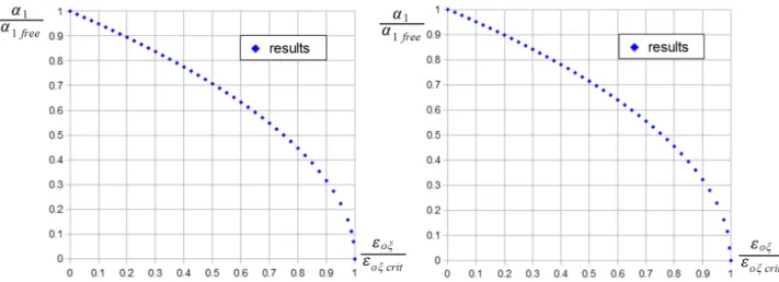
A program has been developed in Fortran90 for solving the eigenvalue problems governed by the Fredholm integral equations. The numerical results have been compared to those valid for the free vibrations of curved beams with the same geometric and material properties. (For more details about the natural frequencies of planar curved beams see [5, 1975].) Figure 2 shoes the quotientα1/α1freeagainst the quotientεoξ/εoξcrit[ Graph (a)]{Graph (b)}shows the results for [the pinned-pinned beam]{the beam fixed at both ends}. It has turned out that the results are independent of both the parametermand the central angle2ϑ. As the loading increases (or what is the same the axial strain grows) the frequencies and therefore the quotients decrease. Observe that there is hardly any noticeable difference between the results for the two support arrangements.

Figure 2. Results for (a) pinned-pinned, and (b) fixed-fixed beams

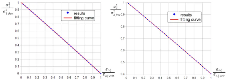
Not less interesting and illustrative are Figures 3 and 4. Considering a pinned-pinned beam Figure 3 represents the quo- tientsα²_i/α²_ifree(i= 1,2)against the quotientεoξ/εoξcrit. In addition to being independent ofmandϑthese relationships are linear with a very good accuracy. Equations

α²₁

α²_{1f ree} = 1.00046−1.00038 ε_oξ εoξ crit

, α²₂

α²_{2f ree} = 1.00204−0.43440 ε_oξ εoξ crit

. (46)

fit onto the computational results with a very good accuracy. The character of these results is the same as that valid for a compressed straight beam if the latter one also vibrates.

Figure 3. Results valid for pinned-pinned beams

The results are incredibly similar for fixed-fixed beams (Figure 4) however a quadratic term shall be added to the approximative polynomials for a better fit:

α²₁

α²_{1f ree} = 1.00190−0.96824 εoξ

ε_{oξ crit} −0.03280 εoξ

ε_{oξ crit} ²

, (47)

α²₂

α²_{2f ree} = 1.00753−0.59031 ε_oξ εoξ crit

−0.0143844 ε_oξ

εoξ crit

2

. (48)

Figure 4. Results valid for fixed-fixed beams 8. CONCLUDING REMARKS

In accordance with our aims we have investigated the vibrations of curved beams with cross sectional heterogeneity subjected to a vertical force at the crown point.

(1) We have derived the governing equations of those boundary value problems which make it possible to clarify how the radial load affects the natural frequencies of the beam.

(2) For pinned-pinned and fixed-fixed beams as well as for beams fixed at one end and pinned at the other end we have determined the Green function matrices assuming that the beams are prestressed by a radial load. Since the length of the paper is limited details were mainly presented for the pinned-pinned beam.

(3) Making use of the Green function matrices we have reduced the eigenvalue problems set up for the frequencies to eigenvalue problems governed by systems of Fredholm integral equations.

(4) Numerical solutions were provided. For the loaded beam considered the square of the natural frequencies depend linearly (pinned-pinned beam) or linearly with a good accuracy (fixed-fixed beam) on the axial strainεoξ. With the knowledge of the relationshipεoξ =εoξ(P)we can determine that value ofεoξ which belongs to a given load and then the natural frequency of the loaded structure. Accuracy of the relations (41) and (42)) is, however, to be investigated. This work is in progress.

Acknowledgement: This research was supported in the framework of TÁMOP 4.2.4. A/2-11-1-2012-0001 „National Excellence Program – Elaborating and operating an inland student and researcher personal support system convergence program” The project was subsidized by the European Union and co-financed by the European Social Fund.

REFERENCES

[1] A.E.H. Love.Treatese on the mathematical theory of elasticity. New York, Dower, 1944.

[2] S. Márkus and T. Nánási. Vibration of curved beams.Shock. Vib. Dig., 13(4):3–14, 1981.

[3] P. A. A. Laura and M. J. Maurizi. Recent research on vibrations of arch-type structures.Shock. Vib. Dig., 19(1):6–9, 1987.

[4] P. Chidamparam and A. W. Leissa. Vibrations of planar curved beams, rings and arches.Applied Mechanis Review, ASME, 46(9):467–483, 1993.

[5] G. Szeidl.Effect of change in length on the natural frequencies and stability of circular beams. Ph.D Thesis, Department of Mechanics, University of Miskolc, Hungary, 1975. (in Hungarian).

[6] Ray Lawther. On the straightness of eigenvalue iterations.Computational Mechanics, 37:362–368, 2005.

[7] Gy. Szeidl and L. Kiss:. A Nonlinear Mechanical Model For Heterogeneous Curved Beams. In S. Vlase, editor,Proceedings of the 4th International Conference on Advanced Composite Materials Enginnering, COMAT, volume 2, pages 589–596, 18 - 20 October 2012, Bra¸sov, Romania.

[8] L. P. Kiss. Free vibrations of heterogeneous curved beams.GÉP, LXIV(5):16–21, 2013. (in Hungarian).

[9] Christopher T. H. Baker.The Numerical Treatment of Integral Equations – Monographs on Numerical Analysis edited by L. Fox and J. Walsh.

Clarendon Press, Oxford, 1977.

[10] L. Kiss.Solutions to some problems of heterogenous curved beams. MSc Thesis, Department of Mechanics, University of Miskolc, 2011. (in Hungarian).