1.Introduction NEWHYBRIDWAVELETANDCNN-BASEDINDIRECTTIRE-PRESSUREMONITORINGSYSTEMFORAUTONOMOUSVEHICLES

(1)

hjic.mk.uni-pannon.hu DOI: 10.33927/hjic-2020-18

NEW HYBRID WAVELET AND CNN-BASED INDIRECT TIRE-PRESSURE MONITORING SYSTEM FOR AUTONOMOUS VEHICLES

ZOLTÁNMÁRTON^*1ANDDÉNESFODOR¹

1Research Institute of Automotive Mechatronics and Automation, University of Pannonia, Egyetem u. 10, Veszprém, 8200, HUNGARY

Since the tire pressure has a significant influence on driving safety, even self-driving vehicles need to be aware of their current tire pressures. Two major types of methods for estimating tire pressures exist: direct and indirect methods. In spite of recent advancements in direct Tire Pressure Monitoring Systems (TPMSs), indirect pressure monitoring systems still play a significant role due to their low costs. Indirect systems rely on the processing of signals from wheel speed sensors.

In most cases, a transformation is applied to generate a frequency spectrum from which the tire pressure-dependent eigenfrequency can be extracted. The most accurate methods apply the Fourier transform, but these require the highest computational power. After the spectrum of signals from the wheel speed sensor is created, the eigenfrequency must be extracted. Several methods are available to extract significant frequency components. One of the easiest methods is peak searching, however, it is susceptible to noise. On the other hand, more accurate methods that are less sensitive to noise require more computational power. If a transform that consumes less computational power can be applied, then the freed resources can be used by a better eigenfrequency identification method. In this paper, a Hybrid Wavelet-Fourier Transform and Convolutional Neural Network-based method is presented, which exhibits a promising level of noise tolerance.

Keywords: TPMS, Eigenfrequency, Hybrid Wavelet-Fourier Transform, Convolutional Neural Net- works, Autonomous Vehicles

1. Introduction

The development and spread of autonomous and electric vehicles is about to change everything with regard to the internal structure and operation of cars. However, vehicles will always make contact with the road through tires so tires will continue to play an important role in terms of vehicle safety. The condition of tires is not only dependent on abrasion but on current tire pressures as well. Furthermore, tire pressures influence abrasion in addition to fuel or power consumption [1]. As a result, both the EU and USA have legislated that all new vehicles are equipped with Tire Pressure Monitoring Systems (TPMS) as standard. To achieve safe autonomous driving, the performance parameters of the vehicles must be in accordance with the conditions of the tires, e.g. the driving logic needs to know the current pressure of each tire.

Nowadays, research is being done with regard to active tires which are capable of adapting to weather and road conditions by changing their own tire pressures according to the requirements [2]. On the other hand, active tires are extortionate compared to their passive counterparts, even those equipped with TPMS. An active tire must also include a compressor and be able to transmit the com- pressed air into the tires, which increases not only their

*Correspondence:marton.zoltan@mk.uni-pannon.hu

cost but also their energy requirements. Active tire systems will only be available for high-end vehicles or mili- tary applications. Mainstream and more cost-effective vehicles will continue to use regular tires and be equipped with TPMS.

Two major types of TPMS are available: direct TPMS, which includes a pressure sensor in the tires them- selves, and indirect TPMS, which uses Wheel Speed Sensors (WSS) required by the Anti-lock Braking Sys- tem (ABS), Electronic Stability Program (ESP) and other driving safety systems. The indirect TPMS (iTPMS) can be accomplished by following two techniques. The simplest way is to compare the wheel speed signals from three different pairs, the bigger the tire pressure the bigger the radius of the tire will be. These systems are capable of detecting relative pressure changes and require the results to be filtered in such a way that the driving conditions and maneuvers do not affect the system. Since tires have different radii, these systems require a learning process to be implemented should any of the tires be changed [3]. Nowadays, comparable systems were re- placed by signal processing-based systems and research is being done on model-based systems. Both approaches are based on the fact that a tire is like a complex system made of springs and masses, where each spring-mass pair has its own eigenfrequencies. One of the springs corre-

(2)

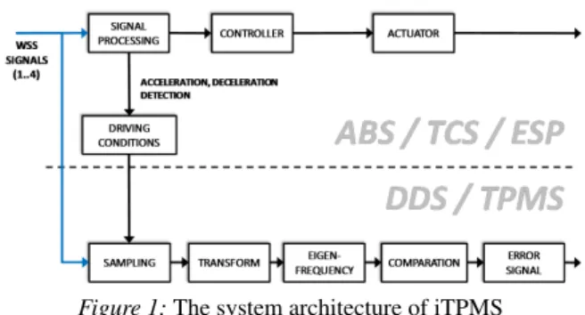
Figure 1:The system architecture of iTPMS

sponds to the air pressure inside the tire, therefore, one eigenfrequency is dependent on the tire pressure [3]. Sig- nal processing-based iTPMSs consist of two major well- separated steps (Fig. 1).

The first step is to transform the signal from the time domain into the frequency or a frequency-related domain.

These transforms can be Fourier [4], Cosine [5] or Hy- brid Wavelet-Fourier (HWFT). The received frequency spectrum of the signal from the wheel speed sensor con- tains different eigenfrequencies as well as noises originating from the road surface, combustion engine and transmission. The second step is to detect and isolate the pressure-dependent eigenfrequency. Different algorithms are available to identify a specific eigenfrequency.

Each algorithm is only performed on a given bandwidth.

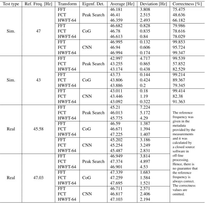
The simplest and fastest is the Peak Search (PS) algorithm. Another method is the so-called Center of Grav- ity (COG) algorithm which can virtually increase the frequency resolution. Although it is more resilient towards noise, noise still may cause the detected eigenfrequency to be shifted. This was subsequently observed in the results presented in Table 1. Since each eigenfrequency found in the spectrum of the WSS exhibits a unique pattern, a pattern-recognition method can also be applied to identify the eigenfrequency in a given bandwidth. One of the most popular and reliable pattern-recognition methods are the deep Convolutional Neural Networks (CNNs).

Deep CNNs can learn to recognize and classify patterns through a process called Deep Learning.

In this paper, a novel iTPMS algorithm is proposed which consists of the HWFT and, as an alternative to the COG algorithm, a CNN is used to detect the eigenfrequency.

2. Transforms related to iTPMS

The first major step in signal processing-based iTPMS is always a transform of the WSS or other sensor signals from a time into a frequency or frequency-equivalent domain. Since one of the major aims of this paper is to compare different transforms and eigenfrequency-detecting methods, a short description will be given of the Fourier, Cosine and Hybrid Wavelet-Fourier transforms. For the iTPMS, a “new” HWFT will be proposed in this paper.

2.1 Fourier Transform

One of the most mainstream transforms in frequency analysis is the Fourier transform, which transforms the time-domain signals directly into the frequency domain [6]. The signals in the frequency domain contain information concerning frequencies, amplitudes and phases.

Three major varieties of the Fourier transform exist depending on the nature of the signal and the number of samples. The Continuous Fourier Transform (CFT) is predominantly used in stability and control theory, signal processing theory, symbolic mathematics, electrical engineering, etc.

If a continuous signal is sampled, i.e. a discrete signal, by using the integral approximation to the sum, the Discrete Fourier Transform (DFT) can be obtained as

X[k] = 1

√ N

N−1

X

n=0

x[n]e^−i2πkn/N, (1) wherekrepresents the discrete frequency, x[n] denotes the sampled signal,Nstands for the number of samples, X[k]refers to the transformed discrete signal andiis the imaginary unit. Unlike the CFT, the DFT has many prac- tical applications.

A special case of DFT is when the number of samples can be expressed as a power of two. In this case, DFT can be factorized using a divide and conquer approach. Hence the factorization of this transform requires less computational power and is referred to as the Fast Fourier Trans- form (FFT), it is the most widespread in signal processing and computer science.

2.2 Cosine Transform

The Cosine Transform (CT) originates from the Fourier transform by removing the imaginary components. Un- like the Fourier transform, where the phases are encoded in the complex amplitudes, the CT stores the phase information over the entire frequency spectrum if the signal cannot be synthesized entirely from a finite set of cosine functions [7]. CT also consists of three major variants: Continuous (CCT), Discrete (DCT) and Fast (FCT).

In practice, FCT is predominantly used in the compression of lossy audio, images and motion pictures. DCT and FCT consist of four different variations, in our case, the so-called DCT or FCT II was implemented:

X[k] =

N−1

X

n=0

x[n] cos

π

k+1 2

n N

. (2) In this paper, FCT was examined as an alternative to FFT.

2.3 Wavelet Transform

The Wavelet Transform (WT) can be seen as a transform which transforms a given signal from the time domain into the frequency-time domain. Like FT and CT,

(3)

Table 1:Test results of different combinations of transform- and eigenfrequency detection methods.

Test type Ref. Freq. [Hz] Transform Eigenf. Det. Average [Hz] Deviation [Hz] Correctness [%]

Sim. 47

FFT

Peak Search

46.181 3.808 75.475

FCT 46.41 2.515 48.636

HWFT-64 46.359 2.493 66.182

FFT

CoG

46.682 0.828 79.986

FCT 46.78 0.835 78.616

HWFT-64 46.613 0.84 78.029

FFT

CNN

46.995 0.132 99.853

FCT 46.94 0.606 95.724

HWFT-64 46.994 0.174 99.347

Sim. 43

FFT

Peak Search

42.997 4.717 99.539

FCT 43.255 0.865 57.852

HWFT-64 43.174 0.438 82.529

FFT

CoG

43.73 0.144 99.214

FCT 43.806 0.424 89.367

HWFT-64 43.886 0.2 79.345

FFT

CNN

43.011 0.18 99.414

FCT 43.446 1.19 82.38

HWFT-64 43.092 0.322 91.363

Real 45.58

FFT

Peak Search

45.21 7.224

The reference frequency was given in the metadata provided by the measurements and it was calculated by a closed source software in off-line processing.

Hence, there is no guarantee that the reference frequency is always correct.

The correctness values are omitted.

FCT 46.013 5.172

HWFT-64 45.775 4.29

FFT

CoG

46.59 1.387

FCT 46.671 1.394

HWFT-64 47.225 1.407

FFT

CNN

45.202 3.186

FCT 45.254 3.249

HWFT-64 45.487 2.831

Real 47.03

FFT

Peak Search

46.949 3.814

FCT 47.374 4.897

HWFT-64 46.901 4.53

FFT

CoG

47.339 1.683

FCT 47.259 1.584

HWFT-64 47.695 1.521

FFT

CNN

46.711 2.571

FCT 46.817 2.406

HWFT-64 47.103 2.194

WT also consists of three variants, namely continuous (CWT):

X(t, s) = 1

√s Z ∞

−∞

x(t)ψ τ−t

s

dt, (3) discrete (DWT):

X[m, k] = 1 pc^k₀

N−1

X

n=0

x[n]ψ n

c^k₀ −m

T

, (4) and fast (FWT), but unlike the aforementioned transforms, WT is not just a transformation, it resembles a whole family of transformations. In the above equations, where ψ(t) is the so-called Mother Wavelet function, x(t)denotes the continuous input signal or function, and X(t, s)represents the WT.

CWT can be discretized. This process requires a scaling basec0and a time unit of the Mother Wavelet,T, to

be defined:

X[m, k] = 1 pc^k₀

N−1

X

n=0

x[n]ψ n

c^k₀ −m

T

(5) If the scaling base is two and the total number of samples can be expressed as a power of two, the previously obtained DWT can be factorized. The obtained FWT can be implemented as a cascade of low pass filters (LPF), high pass filters (HPF) and downsampler banks [8].

Depending on the Mother Wavelet function, different WTs can be defined. These WTs share common properties, e.g. the frequency and time resolutions of the transform are dependent on each other, they can be viewed as bands where both resolutions are in logarithmic steps.

Their other properties depend on which Mother Wavelet is selected. The most widespread WTs are the Mexi- can hat Wavelet, Haar (Wavelet) Transform and Cohen-

(4)

Daubechies-Feauveau (CDF) Wavelets. WTs are applied in data compression, e.g. JPEG2000, DjVu, CineForm, etc., and transient analysis.

2.4 Hybrid Wavelet-Fourier Transform

While WT was applied in signal processing for transient and Fourier transforms in frequency spectrum analysis, demand for both grew simultaneously. One of the solu- tions to meet this requirement was HWFT. The basic idea behind it was that the WT decomposes the signal of the time domain into bandwidths. Inside a bandwidth, char- acteristic information concerning the time domain in the given bandwidth can be found. Therefore, it is possible to perform FTs on each bandwidth [9].

Unlike the Continuous HWFT:

X(f, s) = 1

√s Z ∞

−∞

x(t)π τ−t

s

dt, (6) which is scarcely applied, the Discrete HWFT:

X[f, k] =

N−1

X

m=0

e^{−i2πf m/N} pN c^k₀

N−1

X

n=0

x[n]ψ n

c^k₀−m

T

(7) has some applications in biometry [10]. Fast HWFT (FH- WFT) can be synthesised by applying FFT to the output of each bandwidth of the FWT.

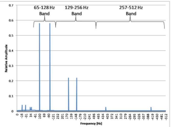
From the perspective of our research, FHWFT is suit- able to calculate a frequency spectrum of a WSS signal for iTPMS applications. Furthermore, FHWFT has a special property which can be exploited to reduce the computational complexity by only performing the FFT on those bandwidths that are significant with regard to the given application. This property allows it to be used as a lightweight alternative to the traditional FFT. How- ever, since the filter banks of the FWT are imperfect, a phenomenon known as spectral leakage can be observed (Fig. 2). Spectral leakage essentially means that frequency components from one bandwidth also appear in the neighboring bandwidths [9]. This causes additional disturbances in the spectrum necessitating further inves- tigation into how much the detection of eigenfrequencies in an iTPMS is affected. For this reason, FHWFT is compared with FFT and FCT using different eigenfrequency detection methods in this paper.

3. Eigenfrequency Detection Methods

The most important step in an iTPMS is eigenfrequency detection because this identifies the frequency component inner pressure dependent. Several methods are capable of identifying or detecting peaks in a given frequency spectrum. The sensitivity, ability to handle multiple peaks, noise susceptibility, etc. of these methods differ.

Figure 2:Spectral leakage of the HWFT demonstrated on a100Hz signal

3.1 Peak Search Algorithm

One of the simplest methods is the Peak Search (PS) algorithm. In the first step, a bandwidth must be determined in which the interesting and/or important eigenfrequencies can be present. In this bandwidth, a search is performed to identify the frequency which exhibits the maximum amplitude. This simple algorithm is presented in

F_p=n f ∈I

max

i |S(i)| =|S(f)|o

, (8) whereF_pdenotes the set of peaks,Irepresents the interval of interest, andS(f)stands for the frequency spectrum of a signal. Under certain circumstances, multiple frequency components can be found. Depending on the application, mostly vibration analysis, error detection as well as searching for local maxima and multiple peaks is required. In such applications, usually a minimum value εis also defined to restrict the number of possible peaks:

F_p={f ∈I||S(f)|>εand||S(f)|is local max} (9) If noise or disturbances are present, the PS algorithm might identify the wrong peaks. To reduce the impact of the noise, a Sliding-Window Median Filter might be applied. If the PS algorithm inEq. 9is used, then it is more resilient to noise than the global maximum method (Eq.

8), but a priori information is required to identify the correct eigenfrequency.

Neither of the PS methods are as accurate in such systems as the iTPMS because pressures about30% lower than the optimum shift the pressure-dependent eigenfrequency by only approximately3−4 Hz. Due to disturbances originating from the road surface and transmission, multiple peaks might be present in the interval of interest.

3.2 Center of Gravity algorithm

A more noise-resistant method is the Center of Gravity (CoG) algorithm since it involves weighted averaging.

(5)

Figure 3:The pressure-dependent eigenfrequency of a tire in the spectrum of the WSS signal

Unlike the PS, COG always yields only one frequency, therefore, this eliminates the problems that originate from multiple peaks present in the Interval of Interest. Further- more, the eigenfrequency theoretically has a higher resolution than would have resulted from the sampling frequency and sampling time. This theoretically increased frequency resolution can only be achieved in the pres- ence of an error and only in that case when exactly one frequency component is present in the Interval of Interest.

The COG can be calculated by fc=

R

If|S(f)|^pdf R

I|S(f)|^pdf , (10) wheref_c denotes the center frequency andprepresents an exponent whose value, depending on the application, is usually between2and3. Although this method is more robust than PS, it is still susceptible to noise.

3.3 Convolutional Neural Networks

The eigenfrequency of the tire exhibits a very distinct pattern in the frequency spectrum of the WSS signal (Fig. 3) which facilitates its detection using pattern-matching algorithms. One of the most popular pattern-matching algorithms involves deep (multilayered) CNNs. Our research focused on developing an algorithm for eigenfrequency detection using CNN. On the downside, CNNs demand much more computational power and memory than PS or COG. To compensate for the higher computational power, a FHWFT was strictly developed to carry out the transform in the bandwidth where the tire pressure- dependent eigenfrequency is located (HWFT-64).

The Artificial Neural Networks (ANNs), e.g., CNN, mimic the structure and supposed operation of neurons and neural systems found in living beings. The differ- ences concern the actual operation of neurons and, unlike the central nervous system of a living being, ANNs often structure Artificial Neurons (ANs) into layers. Since in most cases one layer of neurons is insufficient for most

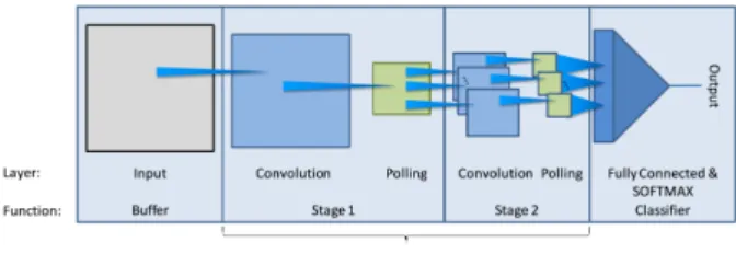
Figure 4:The structure of a simple image classification CNN [12].

applications, multilayer ANNs are often constructed.

ANs often have multiple inputs, each of which has a unique weight assigned to it. Unlike living neurons, the inputs and outputs of ANs can be vector-valued. ANNs store the recognizable patterns in the weight values of their ANs. The analytical determination of the correct weight values is taxing but like the central nervous system of a living being, ANNs can learn the desired patterns. The layers of an ANN can have different functions.

In the case of CNNs, at least one of those layers imple- ment spatial discrete convolution, hence the name Con- volutional Neural Networks. The structure of a layer de- pends on its function as well as the connection between the given layers and the previous layer. Each AN in the layer has a layer-specific Activation Function (AF) which acts as the output function of the AN. Depending on the function of the layer, the following types of layers can be distinguished: input, convolutional, polling and fully connected layer. Since ANs can have vector output values, each layer can be regarded as if each component of the output vector has its own parallel layer with its own weights, which are grouped together as matrices.

The only thing in common would be the AF associated with these virtual parallel layers [11].

Pattern recognition that applies CNNs usually consists of four different types of AN layers: input, convolutional, polling and fully connected (Fig. 4) [12]. The simplest layer is the Input Layer. It has no input weights, moreover, its AF is the identity function and serves as a buffer layer. In the case of Convolutional Layers, each AN shares the same input weights matrices which are referred to as convolution kernels. These layers are applied for noise reduction, filtered downsampling, upsam- pling and feature extraction. The Polling Layer is used for downsampling or dimension reduction of data. Like the Input Layer, it has no input weights but a kernel radius and step distance. Its specific AFs are average, minimum and maximum functions. The Fully Connected (FC) Layer is the most important part of an ANN-based classifier. The number of ANs must be identical to the number of classes the ANN has to distinguish. Its name originates from the fact that each of its neurons are connected to each of the neurons in the previous layer and each connection has a unique weight assigned to it. The ANs in this layer also have a so-called class index attached to them. During the classification, the neurons contain the possibility of their attached classes. This decision can be

(6)

Figure 5:The frequency spectrum of a WSS signal pro- duced by FFT (a) and FHWFT (b) after reordering

influenced by the chosen AF, from which different functions are available. The most commonly used is the so- called softmax function [11].

4. Our New iTPMS Algorithm

4.1 CNN-based Determination of Eigenfre- quencies

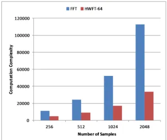
Since similar results can be achieved to FFT using FH- WFT, it can be concluded that FHWFT can be safely used as an alternative to FFT in iTPMSs (Fig. 5). The eigenfrequency, depending on the tire pressure, is between 42 and 48 Hz. Using this information, a FHWFT can be optimized which only calculates the FFT within the bandwidth of 32–63 Hz. If the sampling rate is 1024 samples per second, the FFT has to be performed on only 64 samples. This FHWFT optimized for TPMS was labeled by us as HWFT-64. The computational power requirements of HWFT-64 are about four times less than in the case of a FFT with a sampling rate of 1024 (Fig. 6). The freed up resources make it possible to use more advanced eigenfrequency detection methods than PS or COG algorithms.

Since the CNN can learn different patterns, it is possible to construct such learning patterns which include various frequency disturbances. Naturally, the CNN must also be constructed in such a way that such patterns could be learnt correctly. Furthermore, the CNN should be as simple as possible.

As the first step of the design using the a priori information and by taking the available free and open-source CNN software tool into consideration, an interval of 16 Hz was selected as the interval of interest with 47 Hz (the

Figure 6:Computational complexity of FFT and HWFT- 64

eigenfrequency of the non-deflated tire) at the center. One of the goals of this research was to create a better eigenfrequency detection method than PS. This meant that 16 classes had to be and were specified, thus the last layer of the CNN had to be a fully connected layer that consisted of 16 neurons with a softmax function. Since the input interval is comprised of 16 elements, the input layer also had to consist of 16 neurons. The structure of the pattern recognition-based eigenfrequency-detecting CNN can be even simpler than the simple image classifier shown in Fig. 4since much less input data is used.

The first attempt just applied a two-layer approach, with an Input and an FC Layer. This design could not be validated during the learning process. To enhance the capabilities of the CNN, an additional layer had to be in- serted. The new layer was a Convolutional Layer consist- ing of four neurons and a 3x3 convolution kernel. The outputs were 16D vectors (Fig. 7). The resulting CNN was capable of passing the validation tests and robust against the simulated disturbances. Implementation of the CNN had to be capable of running on an ECU which meant no OpenCL, Compute Unified Device Architecture (CUDA), Compute Shaders or multiprocessor-based implementation could be used. The MOJO-CNN was chosen, which is an open-source implementation with different built in solving algorithms such as Adam, SGD and AdaGrad [13]. Only the Adam solving algorithm was used.

The learning samples were created by frequency shift- ing of the spectrum of a non-deflated tire (Fig. 3). Addi- tional learning samples were created by injecting a spike at 54 Hz because, in most cases, disturbances would oc- cur at this frequency. To prevent overfitting, data augmen- tation was used. The validation samples were slightly al- tered versions of learning samples. The amplitude was al- tered to such a degree of different frequency components that the location of the peaks remained unchanged.

(7)

Figure 7:Structure of eigenfrequency-detecting CNN

After the design of the CNN, the new algorithm was tested. For the tests, FFT, FCT and HWFT-64 were selected as the transforms. The eigenfrequency identification algorithms were PS, COG and our new CNN-based pattern recognition. The test data used consisted of both artificial, referred to as “simulated”, and real measurement data.

4.2 Simulations and Measurements

The first sample tests were conducted in such a way to fa- cilitate a known eigenfrequency. This was accomplished by taking real measurement data, which were filtered by a non-ideal Band-Stop Filter (BSF). The BSF being non- ideal makes it possible for the original frequency components to be still present but attenuated and, therefore, act as disturbances. Following filtration by the BSF, known frequency components were injected (47 Hz and 43 Hz for the non-deflated and deflated tires, respectively).

As previously stated, the other set of test data were unmodified measurement data. The data was provided by Continental AG and the expected eigenfrequency was used as a reference frequency. Two “simulated” and two unmodified measurement sets of test data were used for the tests. During the tests, the average frequency deviation and accuracy were evaluated. The accuracy was defined as how many times the algorithm would yield the reference frequency compared to the number of times the algorithm was executed. This could only be determined on the “simulated” data set, since on real measurements, the eigenfrequency cannot be guaranteed to be always the same as given in the metadata sheet. The noises and disturbances were uncontrolled and originated from the road surface, transmission and combustion engine.

5. Results and Discussion

The results can be seen inTable 1. As can be observed, the CNN yields better results with regard to approach- ing the reference frequency more appropriately and with less deviation than PS and comparable results to COG in the case of both “simulated” and real measurement data.

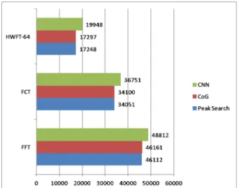
Figure 8:Computational complexity of different combinations of transform- and eigenfrequency-detecting methods, when the number of samples was1024and the interval of interest consisted of16frequency spectral amplitudes

The most significant improvement of the CNN-based pattern recognition method can be observed in the results from the FCT during the “simulated” data tests. How- ever, except for the first test on the 47 Hz “simulated”

data, the COG yielded the smallest deviations, the dif- ferences between the average frequencies of COG and reference frequencies are bigger than in the case of PS or CNN-based pattern recognition methods. In the case of the CNN-based method, the deviation was about50

% greater than in the case of COG. This is most likely due to the fact that the output of the CNN-based method yielded a lower frequency resolution than COG. On the other hand, the HWFT-64 with CNN shows promising and comparable results using just less than half of the computational power required by FFT and COG.

6. Conclusion

In this paper, a new pattern recognition-based eigenfrequency detection algorithm for iTPMS was presented.

By combining this new algorithm with an optimized FH- WFT, the resulting system is of lower computational complexity, moreover, the reliability and accuracy is al- most the same as that of the currently industrial mainstream FFT and COG combination (Fig. 8). The computational complexity was calculated by how often simple mathematical operations supported natively by the CPU/FPU were used in the implementation and how those embedded in iterations were affected by the input data size. In this case, the input data size was1024sam- ples. The COG can also work with the HWFT-64 but is slightly less reliable (Table 1). Since more free resources are still available, when using this new transform optimized for iTPMS, further improvements or more complex eigenfrequency detection methods can be used with- out exceeding the computational complexity of the FFT.

(8)

Acknowledgements

The research was supported by EFOP-3.6.2-16-2017- 00002 programme of the Hungarian National Govern- ment.

REFERENCES

[1] National Highway Traffic Safety Admin- istration, Federal Motor Vehicle Safety Standards, Tire Pressure Monitoring Sys- tems, Controls and Displays, March 2009,

http://www.nhtsa.dot.gov/cars/rules/

rulings/tirepresfinal/TPMSfinalrule.pdf

[2] Schoettle, B.; Sivak, M.: The Importance of Ac- tive and Intelligent Tires for Autonomous Ve- hicles, The University of Michigan Sustainable Worldwide Transportation Report, 2017, Report No. SWT-2017-2 http://umich.edu/~umtriswt/

PDF/SWT-2017-2.pdf

[3] Silva, A.; Sánchez, J. R.; Granados, G. E.; Tudon- Martinez, J. C.; Lozoya-Santos, J. J.: Comparative Analysis in Indirect Tire Pressure Monitoring Sys- tems in Vehicles,IFAC-PapersOnLine, 2019,52(5), 54–59DOI: 10.1016/j.ifacol.2019.09.009

[4] Gustafsson, F.; Drevo, M.; Forssell, U.; Lofgrën, M.; Persson, N.; Quicklund, H.: Virtual Sensors of Tire Pressure and Road Friction,SAE Technical Pa- per Series, 2001.DOI: 10.4271/2001-01-0796

[5] Márton, Z.; Fodor, D.; Enisz, K.; Nagy, K.: Fre- quency Analysis Based Tire Pressure Monitoring,

2014 IEEE International Electric Vehicle Confer- ence (IEVC)DOI: 10.1109/IEVC.2014.7056187

[6] Oberst, U.: The Fast Fourier Transform,SIAM Jour- nal on Control and Optimization, 2007,46(2), 496–

540DOI: 10.1137/060658242

[7] Strang, G.: The Discrete Cosine Transform, SIAM Review, 1999, 41(1), 135–147 DOI:

10.1137/S0036144598336745

[8] Goswami, J. C.; Chan, A. K.: Fundamentals of Wavelets, John Wiley & Sons, Inc., 2011 DOI:

10.1002/9780470926994

[9] Tarasiuk, T.: Hybrid Wavelet-Fourier Spectrum Analysis, IEEE Transactions on Power Delivery, 2004,19(3), 957–964DOI: 10.1109/TPWRD.2004.824398

[10] Ziółko, B.; Kozłowski, W.; Ziółko, M.; Samborski, R.; Sierra, D.; Gałka, J.: Hybrid Wavelet-Fourier- HMM Speaker Recognition,International Journal of Hybrid Information Technology, 2011,4(4), 25–

41

[11] Albawi, S.; Mohammed, T. A.; Al-Zawi, S.: Un- derstanding of a Convolutional Neural Network, 2017 International Conference on Engineering and Technology (ICET), 2017. DOI: 10.1109/ICEngTech- nol.2017.8308186

[12] Hijazi, S.; Kumar, R.; Rowen, C.: Using Convolu- tional Neural Networks for Image Recognition, IP Group, Cadence, 2015.https://ip.cadence.com/

uploads/901/cnn/

[13] https://github.com/gnawice/mojo-cnn/wiki