Are parliaments with more parties cheaper to bribe?
∗Marina Bannikova Universitat Rovira i Virgili †
Attila Tasn´adi
Corvinus University of Budapest ‡ July 16, 2015
Abstract
We collect data about 172 countries: their parliaments, level of corruption, per- ceptions of corruption of parliament and political parties. We find weak empirical evidence supporting the conclusion that corruption increases as the number of parties increases. To provide a theoretical explanation of this finding we present a simple the- oretical model of parliaments formed by parties, which must decide whether to accept or reject a proposal in the presence of a briber, who is interested in having the bill passed. We compute the number of deputies the briber needs to persuade on average in parliaments with different structures described by the number of parties, the voting quota, and the allocation of seats among parties. We find that the average number of seats needed to be bribed decreases as the number of parties increases. Restricting the minimal number of seats a party may have, we show that the average number of seats to be bribed is smaller in parliaments without small parties. Restricting the maximum number of seats a party may have, we find that under simple majority the average number of seats needed to be bribed is smaller for parliaments in which one party has majority, but under qualified majority it hardly changes.
Keywords:Bribing, party composition of a parliament, knapsack problem.
JEL Classification Number: D73, D72.
∗We would like to thank Antonio Quesada for very detailed and insightful comments and suggestions, as well as seminar participants at the Universitat Rovira i Virgili, at the University of Barcelona, and at the Corvinus University of Budapest for helpful remarks. Of course, any errors and shortcomings remain the authors’ responsibility. The first author gratefully acknowledges the financial support from COST Action IC1205 on Computational Social Choice. The second author gratefully acknowledges the financial support from the Hungarian Scientific Research Fund (OTKA K-112975).
†Department of Economics, Universitat Rovira i Virgili and CREIP, Avinguda de la Universitat 1, Reus, Spain, e-mail: marina.bannikova@urv.cat
‡MTA-BCE “Lend¨ulet” Strategic Interactions Research Group, Department of Mathematics, H-1093 Budapest, F˝ov´am t´er 8. e-mail: attila.tasnadi@uni-corvinus.hu
1 Introduction
Voting is the most common procedure by means of which decisions of a group of people are taken, whether it is a nation, a director’s board or a committee. The nation makes a decision about what is the common goal and how to achieve it, a parliament (legislature) is trusted to represent the people’s vision of the joint future of the society. In a modern democracy parties represent groups of people in a parliament.
While the representatives are acting for the sake of social welfare, no problem arises.
But an exogenous agent, a briber, can provide incentives to the representatives to forget their duty and act for the sake of personal profits, which happens less or more frequently depending on the country and may be related to certain relevant characteristics of a parliament. So the question to be studied is which characteristics of the parliament favours the occurrence of bribing in the parliament.
Usually corruption, and bribing as a part of corruption, are studied in a relation to its negative influence on the social welfare of the country, on its economic growth (Mauro (2008), Shleifer and Vishny (1993)), on public investment (Tanzi and Davoodi (1998)), foreign direct investments (Wei (2000)), and on business regulation (Breen and Gillanders (2012), Banerjee (1997), Guriev (2004)).
It seems clear that the level of corruption is influenced by the actual implementation of a representative democracy. Treisman (2000) shows that older democracies foster sig- nificantly lower levels of corruption compared to younger democracies. Later empirical work of Persson, Guido, and Trebbi (2003) reinforced this conclusion. The fundamental components of representative democracy are political parties, a parliament, elections, elec- toral systems, etc. In this field there is a number of studies exploring the elections, voting rules, electoral districts and its vulnerability to corruption and bribing. Myerson (1993) finds that approval voting and proportional representation are fully effective in excluding corrupt parties, plurality voting is partly effective, and the Borda rule voting is ineffective.
His findings were contested by some empirical studies (Persson, Guido, and Trebbi (2003), Rose-Ackerman (2005), and Birch (2007), for instance) and by the later work of Myerson (1999). Specifically, Kunicov´a and Rose-Ackerman (2005) show that proportional represen- tation electoral systems are associated with higher levels of corruption than single-member districts systems. Other studies do not find this relationship significant: for instance, Pers- son, Guido, and Trebbi (2003) show that switching from strictly proportional to strictly majoritarian elections only has a small negative effect on corruption.
Once the parliament is elected, the influence on its decision by exogenous pressure groups is widely studied in the lobbying literature. This literature has identified both a positive and a negative effect of lobbying activities. The positive side is that lobbying groups provide information to policy makers (though there is a clear incentive to furnish only the information that favours the interest of the lobby, so that the decision by policy makers is likely to be biased). The negative side is just based on the fact that lobbying groups may bribe policy makers to decide in favour of their groups. This paper is motivated by this possibility.
The illegal side of lobbying, such as direct bribing, is studied usually in an empir- ical way. For instance, Charron (2011) investigates empirically the connection between party systems and corruption. He finds that multipartism in countries with dominance of single-member districts is associated with higher levels of corruption, while the party sys- tem’s influence on corruption plays no role in countries with proportional representation.
Chang and Golden (2007) find that higher number of political parties makes it difficult for
the public to monitor the behaviour of politicians, and, therefore, corruption increases in multi-party systems. Lederman, Loayza, and Soares (2005) show that democracies, parlia- mentary systems, political stability, and freedom of the press are all associated with lower corruption; and Pelizzo (2006) shows that the potential for corruption is inversely related to the parties levels of institutionalization, that is the more a party is institutionalized, the less likely it is to become involved in corrupt practices.
Dal B´o (2007) presents an interesting game-theoretical model about the influence over collective decisions. In particular, he proves that collusion among voters, such as political parties, and the existence of “disciplinary devices”, such as party discipline, might help to avoid lobbying (or bribing) or “set its price”.
Illegal lobbying procedures take place when interest groups influence a decision through bribes, favours, or promises of future benefits. In our model we deal with the bribing of deputies in order to persuade them to vote for a decision preferred by the briber.
The analysis in our paper is not only motivated by the empirical and theoretical studies listed above, showing that multipartism is associated with high corruption, but also by the data we collected concerning 172 countries. A simple descriptive statistical analysis of the data reveals that parliaments with more parties corresponds to higher level of corruption.
These findings are presented in Section 2. Besides, the study of parliament structures helped us to define the framework of our theoretical model. And more importantly, this empirical exercise raised interesting questions to be answered. What favours bribing in parliament? More or less parties? Greater or smaller election threshold? Equal or unequal allocation of seats between parties? Presence or absence of a majority party?
To answer these questions we propose a simple model to calculate the average bribing cost (measured in members of the parliament) of an exogenous briber interested in having a certain decision approved by the parliament. Comparing the average bribing cost of parliaments different in its structural characteristics, we find that having more parties makes bribing less costly and, consequently, more bribing is likely to occur. Assuming different restrictions on the allocation of seats among parties, we also find that the equal allocation of seats between parties is not always preferred to the parliaments with a more egalitarian allocation; the election threshold reduces the number of seats to be bribed on average; and that the presence of a big ‘dictatorial’ party in parliament only affects bribing under simple majority.
The remainder of the paper is organized as follows. Section 2 contains our empirical findings, while Section 3 describes our theoretical model. The numerical results based on our theoretical model are contained in Section 4. Section 5 concludes our paper. The tables summarizing many of our numerical results are gathered in the Appendix.
2 Stylized facts
Our first aim is to investigate whether the empirical evidence suggests a connection be- tween parliament structure and level of corruption. First, we collected data for 172 coun- tries about their parliaments and level of corruption. Our attention is focused on year 2011, since this is the most recent year for which all the sources provide the most com- plete information.
It is difficult to define corruption and bribing. Moreover, as corruption and bribing generally are illegal, violators try to keep it secret. Furthermore, based on culture and traditions, what in one country is considered to be illegal bribing, in another country might be seen as a social norm. There are some debates on how corruption should be measured
(see, for instance, Svensson (2005)). As the general indicator of corruption we decided to take the World Governance Indicator of Control of Corruption (WGICC), provided by the World Bank. It is an aggregate indicator that reflects “perceptions of the extent to which public power is exercised for private gain, including both petty and grand forms of corruption, as well as ‘capture’ of the state by elites and private interests”. The range is from −2.5 (low control of corruption) to 2.5 (high control of corruption). Since we are interested in bribing and corruption inside of the parliament, we selected two indicators, provided in the Global Corruption Barometer by Transparency International: Perceptions of corruption of political parties (PP) and perceptions of corruption of parliament (PL).
These indexes are showing the perceptions of people about the extent to which some constituents of their democratic system are affected by corruption. For year 2011 these indexes are available for 98 countries of our sample. The indexes range from−5 (extremely corrupt) to −1 (not at all corrupt). For simplicity, since “the greater is the index the less there is corruption” we had to invert these indicators, which originally ranged from 1 (not at all corrupt) to 5 (extremely corrupt).
If the parliament is bicameral, only the lower house is taken into account. The size of parliament equals the number of representatives forming the parliament. In almost 70%
of the countries (116 countries) there are no independent representatives. In 56 countries (32.5 %) there are independent deputies. In Table 1 the basic descriptive statistics are presented for the total sample and separately for these categories.
Table 1: Descriptive statistics of parliament characteristics and corruption level in 172 countries. Year 2011.
Total No independent deputies Independent deputies
Variable Number of
countries Mean Number of
countries Mean Number of
countries Mean Size of the Parliament
(number of seats) 172 216.10 (*) 116 206.30 (**) 56 236.30
Number of parties 172 8.73 116 7.27 56 10.77
Number of indepen-
dent deputies 172 6.50 116 0 56 19.9
World governance indi-
cator (WGICC) 172 −0.077 116 −0.060 56 −0.364
Perceptions about cor- ruption of political par- ties (PP)
99 −1.26 60 −1.23 39 −1.32
Perceptions about cor- ruption of parliament (PL)
99 −1.50 60 −1.52 39 −1.46
Without the parliament of China, the average size would be 200 (*) and 182 (**)
On average a parliament consists of around 216 seats. It is worth mentioning that the Chinese parliament consisting of 2987 deputies has an extremely large number of representatives. Excluding China from the sample, gives almost 200 seats on total average and 182 seats on average among those parliaments without independent deputies (without significant change in other variables). It may be inferred from the data, that generally, big parliaments tend to have independent deputies.
On average the number of parties is 8.73, half of the countries have no more than 6 parties (5 and 8 for parliaments without and with independent deputies, respectively). In the whole sample India has the maximum number of parties with 37 parties. In parliaments without independent deputies the maximum number of parties can be found in Chad with 31 parties.
In 56 countries of the second group of countries having independent deputies on average there are almost 20 independents. Half of these countries have no more than 8 independent deputies. There are some extreme cases, such as Afghanistan with 164 independents and 20 parties, Belarus with 125 independents and 3 parties in a parliament of 125 seats, and Syria with 81 independents and 11 parties. There is the problematic issue of how to treat independent deputies: each as a separate party or as a party called “others” with(out) party discipline? We have decided to restrict our attention to 116 parliaments formed only by parties.
Since it is well studied that corruption and bribing are negatively correlated with income (see, for instance, Mauro (2008), Shleifer and Vishny (1993), Tanzi and Davoodi (1998)), we divide these countries in four groups by income level using the classification provided by the World Bank. Table 2 shows the averages values for these four groups of countries.
Table 2: Parliament structure and corruption: averages by income level groups. Year 2011.
Variable High income Upper middle
income
Lower middle
income Low income
Size of the parliament (number of seats) 213.61 260.57* 184.100 147.727
Number of parties in the parliament 6.58 6.89 7.82 8.45
World governance indicator of control of
corruption 1.210 -0.097 -0.527 -0.807
Perceptions of corruption of political par-
ties −3.686 −3.982 −3.8274 −3.367
Perceptions of corruption of the parlia-
ment −3.231 −3.847 −3.553 −3.133
Number of observations 33 37 28 18
* Without the parliament of China, consisting of 2987 representatives, the average size would be 184.83.
Higher income countries on average have fewer parties than lower income countries.
The size of parliament in the Upper middle income group is biased due to the parliament of China: without it the average size of the parliament would be 181.54 (with almost no change in the other variables), and the resulting conclusion is that on average the parliament is bigger in higher income countries. This conclusion can be explained by the fact that higher income countries (with some exceptions) have been enjoying the democracy for longer, so that parliaments may be bigger in order to better represent the views of the citizens. At the same time the average number of parties is smaller in higher income countries, what can be explained by the fact that, in the long run, the small parties do not eventually survive or form coalitions to be more effective.
On average the political parties and the parliament are perceived to be highly corrupt in upper middle income countries (-3.98 and -3.85, respectively) and are perceived least
corrupt in low income countries (-3.37 and -3.13, respectively), but the difference is not as crucial as for WGCC.
Stylized fact 1. In high income countries parliaments are bigger, and with fewer parties.
In low income countries parliaments are smaller, with more parties,but these parties are not perceived so much as corrupt as in the others income groups.
High income countries enjoy the strongest control of corruption (1.21 on average) while the low income countries experience weak control of corruption (-0.87 on average). This empirical evidence is confirmed by the already mentioned studies.
Stylized fact 2. There is a strong positive correlation between control of corruption and income of a country.
Figure 2 illustrates this fact and addresses the question of whether the control of corruption decreases with the increase of number of parties.
Figure 1: World Governance Indicator of Control of Corruption correlated with number of parties for 116 countries grouped by income level into four groups.
In all groups except the high income group there is a decrease of control of corruption showed by linear fitted values. In high income countries democracy was established time ago, and has become more mature. With the development of democracy parliamentary parties become more efficient, stable, and start to form coalitions, but after some time, more parties more focused on specific issues begin to appear, such as Party for the Animals in Parliament of Netherlands; Animal Justice Party in New South Wales Legislative Coun- cil (Australia); Green parties, etc. Such parties are hardly known in low income countries.
So, the conjecture is that a more developed democracy tends to produce a small increase
in the number of parties, because in mature democracies most big issues have been re- solved (or there is an agreement on them among most parties) and citizens may start worrying about issues or problems which are secondary (like animal rights), or viewed as less important, in young democracies.
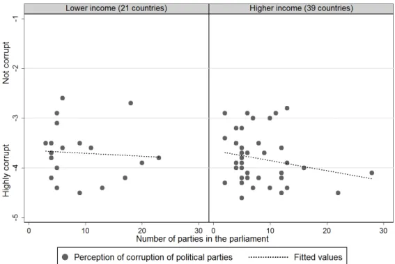
Figure 2: Perception of corruption of political parties correlated with number of parties for 116 countries grouped by income into 4 groups. Year 2011.
Due to a small amount of observation for indexes PP and PL, we merged the four income groups into two groups: “lower income” (21 countries) and “higher income” (39 countries). Both groups show that the greater is the amount of parties in the parliament, the more the parliament and political parties are perceived as corrupt.
Stylized fact 3. In countries with more parties in the parliament people seem to perceive the parliament and the political parties to be more corrupt, especially, in high-income countries.
3 The Model
We consider a given parliament. We shall denote by m the number of parties in the parliament, byn the number of seats in the parliament and byt the minimum number of favourable votes required to pass a bill. Furthermore, we shall denote byM ={1, . . . , m}
the set of parties and by n1, . . . , nm their respective number of representatives. Hence, Pm
i=1ni =n andni ≥1 for alli∈M.
We assume that there is party discipline, that is, concerning any bill each representative of a party votes in the same way. Besides simplifying our calculations, our assumption of
Figure 3: Perception of corruption of the parliament correlated with number of parties for 116 countries grouped by income into 4 groups. Year 2011.
party discipline can be partially justified by the observation (see, for instance, Bowler, Far- rell, and Katz (1999)) that in many countries, especially in case of important issues, after party internal discussions all representatives of a party vote in the same way. Therefore, in our model parties are the decision makers and vote with either yes or no, henceforth briefly denoted by Y orN. The parties’ initial decisions will be denoted byd1, . . . , dm∈ {Y, N}, which might be determined by parties initial political ideological standpoints, while the set of parties initially supporting a bill will be denoted byD={i∈M |di =Y) and the respective number of their representatives by nD =P
i∈Dni.
Since we aim at establishing a connection between the number of parties and the vulnerability with respect to corruption, we will admit several sets of possible allocations of seats and all possible initial decisions for a givenm,nandtinto consideration. We may restrict the set of all possible allocations of seats by a lower bound L and by an upper bound U on party sizes to obtain a possibly restricted set of admissible seat allocations, where we will denote the respective set of admissible seat allocations and all possible initial decisions by
Ωmn(L, U) = (
(n1, . . . , nm, d1, . . . , dm)∈ {1, . . . , n}m× {Y, N}m |
m
X
i=1
ni =n, L≤ni ≤U )
and we will refer to an ω ∈Ωmn(L, U) as a possible state of a parliament. In most of the cases the set of states will be relatively large because we do not want to restrict ourselves to already observed seat distributions in the past since in the future any admissible seat distribution might be possible. The set of all possible allocations of seats, which we also call the unrestricted case, can be obtained by setting L= 1 and U =n−m+ 1, meaning
that each party at least has 1 seat and can occupy a maximum of n−m+ 1 seats, which guarantees that each party has at least one seat.
For a given allocation n1, . . . , nm of seats among parties, and initial decisions d1, . . . , dm, a briber may consider to bribe parties in order to get a bill passed if it did not obtain already sufficient support, that is, ifnD < t. We assume for simplicity that the cost of bribing a party (i.e. to turn its initial N to Y) is proportional to its number of repre- sentatives, and therefore we measure the associated cost of bribing by its size. Assuming bribing costs proportional to the sizes of parties, is a natural starting assumption in case of lack of further information. Clearly, factors like parties initial commitments to their initial decisions or sizes of parties have an affect on bribing costs in a more general way.
However, trying to incorporate these additional factors, would increase the number of free parameters in our model, which also would critically slow down computing bribing costs.
Therefore, for a given allocation of seats and for given initial decisions ω∈Ωmn(L, U) the cost of bribing, which we shall denote byβ(ω), is determined by the following problem:
β(ω) = min (
X
i∈I
ni |I ⊆M\D and X
i∈I
ni ≥max{t−n0,0}
)
. (1)
There are several links to the literature on power indexes and the way how we formulated the briber’s problem (1): While functionβ is single-valued, it would have been possible to define values for each parties by the minimization problem (1), that is to introduce a new power index by determining the number of cases in which a party collects a bribe or the amount it receives by taking the average values of the respective solutions of problem (1);
and therefore obtaining a modified, restricted, and weighted Deegan and Packel (1978) power index. The obtained power index would be modified in the sense that minimal winning coalitions would be replaced with minimum winning coalitions, restricted in the sense that parties from set D would be excluded from the calculations, and weighted in the sense that seats would serve as weights. We will consider the respective power indexes in a separate paper since this is not our purpose here because we are only interested in the briber’s cost.
Instead of assuming that the cost of bribing a party is proportional to its number of representatives, another possibility would have been to assume that the cost of bribing a party was proportional to its power index. However, this would have raised two problems:
the choice of the appropriate power index and an extreme increase in computation time since determining power indexes is a computationally complex task, as it has been shown by Matsui and Matsui (2001).
In a similar spirit to Laruelle and Valenciano (2002) in case of power indexes we allow for all possible decisions of parties, and we assume that any admissible state emerges with equal probability, which is a particular case in Laruelle and Valenciano (2002). Hence, we define the average bribing cost by
AV Gmn(L, U) = P
ω∈Ωmn(L,U)β(ω)
#Ωmn(L, U) , (2)
Replacing the uniform distribution above the set of admissible states, would require fur- ther empirical analysis and result in a dramatic increase in the number of parameters in a modified version of expression (2) as well as a critical computational slow down in its eval- uation. Looking at problems (1) and (2), we can see that parties do not act strategically since we take all possible profiles of party decisions into consideration. Thus, our problem
is of combinatorial nature. It can be verified that the cardinality of Ωmn(1, n−m+ 1) in the unrestricted case equals m−1n−1
2m, which makes a brute force algorithm quite time consuming. Luckily the brute force algorithm enabled us to determine average bribing costs for up to 10 parties within an afternoon. The main steps were generating all pos- sible allocations of seats (where we have taken symmetries into account to speed up the procedure), generating all possible initial decisions and then solving problem (1) by brute force.
To determine the computational complexity of calculating the average bribing cost, we will need the recognition version of the famous knapsack problem, which was shown to be NP-complete by Karp (1972). The knapsack problem is specified in the following way: Consider a knapsack that has a limit weight of W ∈ Z+, which can be filled with m objects of weights w1, . . . , wm ∈Z+ and respective valuesv1, . . . , vm ∈Z+. The target goal is to pick a subset of objects I ⊆M such that their total value is at least V ∈Z+. The knapsack problem asks whether there exists a set I ⊆ M such that P
i∈Iwi ≤ W and P
i∈Ivi ≥ V. From Papadimitriou (1994, p. 202) we even know that the problem is already NP-complete if vi = wi for all i ∈ M and V = W. Now we can check that the recognition version of problem (1) is NP-complete. In the recognition version of problem (1) minimizing bribes is replaced with the question of whether passing the bill is feasible by bribing at most a given number of b representative, i.e there exist anI ⊆M\D such that
X
i∈I
ni ≤band X
i∈I
ni ≥max{t−n0,0}. (3)
Hence, in order to obtain a polynomial time reduction from the restricted version of the knapsack problem to problem (3) let D = ∅, ni = vi for all i ∈ M, t = V and b = V. Therefore, if P6=NP, then a polynomial time algorithm for solving problem (1), and thus also for solving problem (2) does not exist.
4 Results
We provide the results of the calculations for a parliament of 100 seats formed by a number of parties ranging from 2 to 10. We restrict the number of parties for computational reasons. For instance, for 10 parties there are more than a quadrillion of possible states of the world, in each of them an optimal decision has to be chosen. The data from Section 2 show that on average there are 7 parties in parliaments without independent deputies, half of the countries have no more than 5 parties and 77% has no more than 10 parties, so the restriction of 10 parties seems to be reasonable and justifiable.
We provide the results for each possible voting quota 1 ≤ t ≤ n, but mostly we concentrate our attention on majority rules, such as simply majority, two thirds, three fourths, four fifths majority, and unanimity.
There are 4 cases to be considered depending on the restrictions on the party size:
• All party sizes are possible, which we call the unrestricted case,
• Similarly sized parties,
• Without small parties,
• Without big parties.
The first case is the most general one in which any allocation of seats between parties is possible.
The second case is motivated by the analysis of the allocation of seats among par- ties in 172 countries, which indicates that in some parliaments seats are divided almost equally between parties. The two-party parliament of Malta provides a perfect example:
After general elections in 2008, out of 69 seats, the Nationalist Party got 35 seats and Malta Labour Party got 34 seats. We might compare political parties competing for seats with firms competing for a market share. On many product markets we can observe an increasing level of concentration, i.e. having fewer and fewer ‘non negligible’ firms on the market. The same logic can be applied to the “political market”, where the firms are the parties and the consumers are the voters. Besides, some voting procedures favour the emergence of big parties; so the small parties are given incentives to form federations and run elections together. For example, the Catalan party CiU, which was a federation of two constituent parties, the Democratic Convergence of Catalonia and the Democratic Union of Catalonia.
Case 3 is motivated by the existence of the restriction for parties (or candidates from a party) to run the elections. For example, in the United Kingdom a candidate for the parliamentary election is required the present a signed assent of ten registered electors plus a deposit of £500 which is forfeited if the candidate wins less than 5% of the vote.
A typical restriction for entering parliament is to pass a certain threshold level of vote share ratio. Usually the election threshold is 5-7%, in some countries a threshold of 10% is implemented. In a purely proportional electoral system in a parliament of 100 seats 1 seat represents approximately 1% of votes. Furthermore, an election threshold of 5% means that no party occupies less than 5 seats.
Case 4 is motivated both by empirical evidence and by the symmetry with the Case 3. In 55 countries out of 116 (i.e. 47 %) there is a party which occupies the majority of the seats. In 24 countries there is a party with more than 70% of the seats. In 13 of the countries there is a party with more than 80% of the seats. And in 8 countries there is a party which occupies more than 90% of the seats. Another motivation is as follows. If it is relevant to impose a lower limit on parties’ vote share ratio (or have another rule which eliminates small parties), why not put an upper limit? Though there are no such limits in practice, it would be interesting to see what its affects would be.
4.1 Unrestricted case
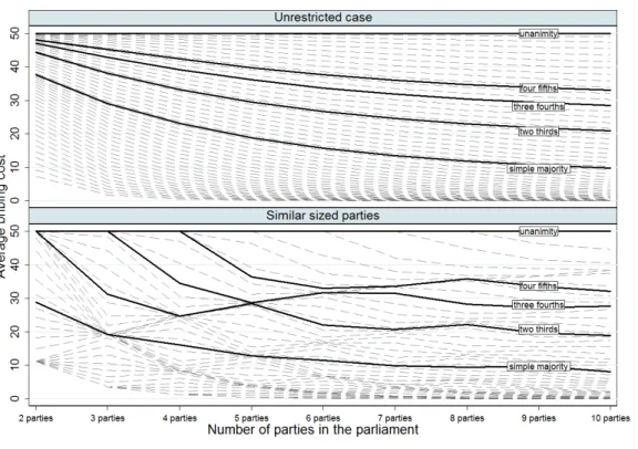
The average bribing cost decreases with the increase in the number of parties, as it is illus- trated in Figure 4. Maximum average bribing cost (50 seats) is achieved under unanimity for all the number of parties, which is obvious, since positive and negative decisions are equally likely. The decrease slows down with the increase in the number of parties and with the increase in the required level of support. The 2-party parliament appears to be the least vulnerable to bribing.
It is interesting to notice that the average bribing cost of a parliament with less parties can be replicated in a parliament with more parties by changing the voting rule. For instance, under simple majority the average bribing cost of the 2-party parliament is 37.2 seats, while for the 3-party parliament it is 29 seats. By changing the voting rule from simple majority to two thirds, the average bribing cost becomes 37.6 seats for the 3-party parliament. Such a change seems to be an extremely large one. But for more parties such a major change is not required. For instance, under simple majority the average bribing cost
Figure 4: Average number of members of parliament of 100 seats needed to be bribed in order to achieve a positive decision (average bribing cost) for unrestricted and similarly sized allocations of seats among 2-10 parties for different voting quotas.
for a parliament with 7 parties is 13.5 seats. To replicate this cost in a parliament with 8 parties it is enough to increase the voting threshold from 51 to 53, where the average bribing cost would be 13.7 for a parliament with 8 parties. All these observations and in the overall Figure 4 gives us the following result.
Result 1. If in a parliament with at most ten parties all possible seat allocations are equally likely, then for any voting quota necessary to reach a decision the average bribing cost decreases as the number of parties increases.
Generally, the policy makers (or “designers” of the parliament) might be interested in restricting access of parties to the parliament, or in forcing parties to form coalitions and, therefore, decrease the number of parties in order to increase the cost of bribing, and thus reduce corruption.
4.2 Parliaments with similarly sized parties
We now restrict our attention to parliaments with similarly sized parties. To do so we impose different lower and upper bounds on the party size by allowing a different degree γ of variation from the egalitarian allocationni =n/m:
L=jn m −γ n
m k
, U =ln m +γn
m m
(4)
jn m −γn
m k
≤ni≤ln m +γn
m m
(5) The special case ofγ = 0% will also be called the equally sized case.
On Figure 4 the result forγ= 20% is presented along with the unrestricted allocation.
Results for different degrees of size variations are presented in Table 4. Results for unanim- ity remain the same as under unrestricted allocation. For simple majority it is true that the average bribing cost decreases with the increase in the number of parties. Under sim- ple majority average bribing cost in parliaments with 3-9 similarly sized parties is smaller than average bribing cost in parliaments with more parties for the unrestricted case. For a parliament with 2 parties it holds for weak (γ >5%) restrictions on the equality of parties, and does not hold for strong (γ ≤5%) restrictions.
But for the qualified majority rules the average bribing cost does not always decrease with the increase of number of parties. For instance, under two-thirds majority, the average bribing cost increases when we pass from a parliament with 4 parties to a parliament with 5 parties. In this case it might be preferred to encourage more parties to appear in order to pass from 4 to 5, and therefore to increase the average bribing cost. This example for 5 parties and obtained results (see Table 4) give us the next result.
Result 2. If the allowed seat allocations of a parliament with at most ten parties are those in which parties do not differ ”much” in size from each other, then:
(a) the average bribing cost still monotonically decreases in the number of parties when decisions are taken by simple majority;
(b) when some form of super majority is required to make a decision, the average seems to be eventually decreasing but may increase depending on the number of parties.
Consider a particular example of 5 parties and the most frequently applied rules:
Simple majority and two-thirds majority. Different γs produce different size restrictions.
The ideally equal allocation would be that each party occupies exactly 20 seats: γ = 0%.
By increasing γ we relax the restriction up to 10≤ni ≤30, when γ = 50%. Kyrgyzstan and Latvia provide nice examples of similarly sized allocation of seats between parties in 2011:γ = 41% (28,26,25,23,18), andγ= 52% (31,22,20,14,13), respectively. Austria can be considered as an example of an extremely relaxed similarly sized allocation: γ = 186%
(57,51,34,21,20).
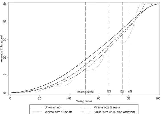
Figure 5 shows that under simple majority the unrestricted allocation is more costly than all the possible similarly sized allocations, but under the two-thirds rule it performs worse than a 10% size variation as well as an equal allocation.
As a justification, the six-party parliament with unrestricted allocation is presented.
For simple majority it is more costly than all the similarly sized allocations between five parties. Hence, it might be the case that under simple majority policy makers would rather prefer to encourage a new party to come in (or to lower the election threshold in order to allow one more party, though a small one, to enter parliament). But if the two-thirds rule is used, this would decrease the average bribing cost instead of increasing it.
4.3 Parliaments without small parties
In this subsection we compute the average bribing cost for parliaments without small parties. We restrict the minimal number of seats which a party needs to occupy: L = 5
Figure 5: Average number of members of parliament of 100 seats needed to be bribed in order to achieve a positive decision (average bribing cost) for 5 similarly sizes parties.
seats, L = 10 seats. The lower bound can be seen as an election threshold: A certain percent of votes a party has to have in order to enter to the parliament.
At first glance, it seems that eliminating small parties would increase the average bribing cost. First, the number of states #Ωmn decreases. Second, no small parties to be bribed means that the briber will be bribing more excessive seats, than he needs: β(ω) increases. But it appears that there are less states when the briber needs to act, therefore though some of the components of the sum P
ω∈Ωmn β(ω) are greater, but the sum itself gets smaller with the elimination of small parties.
On Figure 6 average bribing cost for different election thresholds (lower bounds) in a parliament with 5 parties is presented. It is easy to see that for all majority rules the average bribing cost decreases with the increase of the lower bound. Note that in this case under a simple majority for a parliament with 5 parties and a lower bound of 10 seats the average bribing cost is 13.3 seats, which is smaller than for a parliament of 6 or 7 parties and unrestricted allocation, where the average bribing cost is 15.7 and 13.5 seats, respectively (see Figure 4 and Table 5). For all parliaments with more than 5 parties the same conclusion holds: Average bribing cost in a parliament without small parties is greater than in parliaments with one more party in the unrestricted case. So, it might be the case that for a parliament with more than 5 similarly sized parties the corruption cost can be increased if one more party enters to the parliament in order to deter the briber.
For parliaments with less than 5 parties this does not hold for qualified majority rules.
Result 3. If the admissible seat allocations of a parliament with at most ten parties are
Figure 6: Average number of members of parliament of 100 seats needed to be bribed in order to achieve a positive decision (average bribing cost) for 5 parties occupying not less than 5 (10) seats.
those in which parties cannot occupy less than a certain number of seats (5 or 10 seats, for instance), then the average bribing cost decreases in the minimally required number of seats.
The restriction L = 10 means that if there are 10 parties in the parliament, all the parties have exactly 10 seats. And this makes average bribing cost greater than for a parliament with 9 or 8 parties. More details can be seen in Table 5 in the Appendix.
4.4 Parliaments without big parties
If there is a lower limit why there are no upper limits? Of course, generally, if there is a big party in a parliament, it reflects the views of the majority of the voters, so such a restriction is not fair with respect to the views of the citizens. But the question is: Why do we care about the representation of the views of the voters when we allow a big ‘dictatorial’
party and at the same time neglect the full representation of the views when we establish the election threshold? Might be if society considers necessary to restrict the entrance of small parties, it might consider also to restrict the ‘dictatorship’ in parliaments.
In this subsection we compute the average bribing cost restricting the upper bound.
The softest restriction is that no party has more than 70% of the seats: U = 70. The strongest restriction is that no party has a majority of the seats U = 50. The results for 5 parties are presented on Figure 7.
Figure 7: Average number of members of parliament of 100 seats needed to be bribed in order to achieve a positive decision (average bribing cost) for 5 parties occupying not more than 70 (60 and 50) seats.
Under simple majority the average bribing cost decreases, that is a presence of a
‘dictatorial’ party makes bribing easier. But under qualified majorities even the strictest demand “no party has more than 50% of seats” hardly makes a difference.
In a parliament with several parties the requirement that no party has a majority eliminates not a big part of the states of the world. But in a 2-party parliament it means that all the allocations except (n1, n2) = (50,50) are eliminated. The condition U = 60 actually refers to the case of similarly sized parties in the parliament: no party occupies less than 40 or more than 60 seats. So, consider a parliament with 3 parties. The requirement U = 50 eliminates quite a part of the states of the world.
The average bribing cost for a 3-party parliament under upper bound restrictions are shown on Figure 8. Under simple majority the average bribing cost gets smaller as the upper bound restriction gets smaller. The strictest case “no party has a majority”
decreases the bribing cost from 29 seats to 17.8 seats. For the two-thirds rule there is almost no difference. And for the other qualified majorities the cost slightly increases the smaller is the upper bound.
For instance, the restrictionU = 50 means that either there is no ‘small party’ (with at most 20 seats) or there is one small party. If four fifths is required, in case of no small party it means that if there is one party voting positively, #D = 1, then to reach the quota, the briber has to bribe both parties. If #D= 2, the briber still has to bribe 1 more party. In the worst case #D = 0 the briber has to bribe the 3 parties in order to reach
Figure 8: Average number of members of parliament of 100 seats needed to be bribed in order to achieve a positive decision (average bribing cost) for 3 parties occupying not more than 70 (60 and 50) seats.
the quota. If there is a small party and one of the non-small parties votes Y, the briber has to bribe the other non-small party, because with bribing the small party he will not reach the quota.
Our numerical calculations (also see Table 6) give us the following results.
Result 4. If the admissible seat allocations of a parliament with at most ten parties are those in which parties do not occupy more than a certain number of seats (e.g. 50, 60, or 70 seats), then:
(a) the average bribing cost decreases with the increase of maximum size when decisions are taken by simple majority;
(b) when some form of super majority is required to make a decision, the average bribing cost does not vary when different restrictions on maximum party size are applied.
5 Conclusions
The literature has been mostly concerned with correlating income level of the country with its democratic development, including parliaments and with levels of corruption and bribing. The connection between bribing and parliaments is usually considered at the moment of general elections, from the point of view of simple voters and bribing their
votes. However, in this paper we tried to analyse the bribing once the parliament is already elected. First we collected some empirical data about 172 countries. It showed that in high income countries parliaments are bigger, with fewer parties; in low income countries parliaments are smaller, with more parties. Higher income countries show stronger control of corruption, but the parliament and political parties are perceived to be corrupted as much as in lower income countries, which have weaker control of corruption.
Under the assumptions that each party votes ”yes” or ”no” with equal probabilities and that all possible allocations of seats between parties are equally likely, the result tells that more parties in the parliament decreases the number of seats to be bribed for both simple and qualified majority rules. The decrease is smaller for greater number of parties. The average bribing cost of a parliament with less parties can be reproduced in a parliament with more parties by increasing the voting threshold. And the greater is the number of parties, the smaller is the required change.
In a parliament with similarly sized parties the average bribing cost increases in the number of parties only under the simple majority rule. For qualified majorities there is no general conclusion, though we can define average bribing cost for different parliaments.
Comparing the unrestricted case with similarly sized parties it appears that there might be the case when encouraging one more party to enter the parliament increases significantly the average bribing cost.
Under simple majority average bribing cost in parliaments with 3-9 similarly sized parties is smaller than the average bribing cost in parliaments with more parties in the unrestricted case. For a parliament with 2 parties it holds for weak (γ >5%) restrictions of equality of parties, and does not hold for strong (γ ≤5%) restrictions.
In parliaments without small parties the average bribing cost gets smaller with the increase of the lower bound of party size. In a purely proportional system it can serve as a proxy for an election threshold to enter parliament. Hence, the conclusion is that the election threshold makes bribing less costly for both simple and qualified majority rules.
Under simple majority the average bribing cost is smaller for parliaments without a big ‘dictatorial’ party: the greater is the restriction for the maximum size of a party, the smaller is the average bribing cost. Under qualified majority for parliaments with more than 3 parties, average bribing cost almost does not change if the maximum party size is restricted. And in parliaments with 2 or 3 parties it even gets greater for strict qualified majority rules.
For future research the proposed model can be extended to answer several more ques- tions. To be more realistic, the parties should differ between each other not only in the number of seats in parliament, but also in their political views. Assume that we have a strong right wing party and a “Yes” answer favours the left wing. Such a party is likely to be never bribed for a “Yes” decision, or, in other words, the price to be paid for each seat will be much higher than for a central party or a right wing party with more liberal views. Therefore, for a specific question we can define a bribing propensity a measure of the likelihood to accept a bribe. And even if there are two equal parties in their political views, one can be more corrupted than the other.
It would be nice to see if relaxing party discipline changes the result. The conjec- ture is that hardly, since there will be a “model-in-the-model”: Each partyi represents a parliament with m=ni parties.
The most difficult extension seems to be relaxing the assumption on uniform distri- bution above the set of admissible seat allocations among parties, which would require
additional empirical studies to identify the underlying distribution.
References
Banerjee, A. V. (1997): “A Theory of Misgovernance,”The Quarterly Journal of Eco- nomics, 112(4), 1289–1332.
Birch, S. (2007): “Electoral Systems and Electoral Misconduct,” Comparative Political Studies, 40(12), 1533–1556.
Bowler, S., D. M. Farrell,andR. S. Katz(1999):Party discipline and parliamentary government. Ohio State University Press.
Breen, M., andR. Gillanders(2012): “Corruption, institutions and regulation,”Eco- nomics of Governance, 13(3), 263–285.
Chang, E. C. C., and M. a. Golden (2007): “Electoral Systems, District Magnitude and Corruption,”British Journal of Political Science, 37(December 2006), 115.
Charron, N. (2011): “Party systems, electoral systems and constraints on corruption,”
Electoral Studies, 30(4), 595–606.
Dal B´o, E. (2007): “Bribing voters,”American Journal of Political Science, 51(4), 789–
803.
Deegan, J., J., and E. Packel (1978): “A new index of power for simplen-person games,” International Journal of Game Theory, 7(2), 113–123.
Guriev, S. (2004): “Red tape and corruption,” Journal of Development Economics, 73, 489–504.
Karp, R.(1972): “Reducibility among Combinatorial Problems,” inComplexity of Com- puter Computations, ed. by R. Miller, J. Thatcher,andJ. Bohlinger, The IBM Research Symposia Series, pp. 85–103. Springer US.
Kunicov´a, J., and S. Rose-Ackerman (2005): “Electoral Rules and Constitutional Structures as Constraints on Corruption,”British Journal of Political Science, 35(2005), 573.
Laruelle, A., and F. Valenciano (2002): “Power indices and the veil of ignorance,”
International Journal of Game Theory, 31(3), 331–339.
Lederman, D., N. V. Loayza, and R. R. Soares (2005): “Accountability and Cor- ruption: Political Institutions Matter,”Economics & Politics, 17, 1–35.
Matsui, Y., and T. Matsui (2001): “NP-completeness for calculating power indices of weighted majority games,”Theoretical Computer Science, 263, 305–310.
Mauro, P. (2008): “Corruption and Growth,” Quarterly Journal of Economics, 110(3), 681–712.
Myerson, R. B. (1993): “Effectiveness of Electoral Systems for Reducing Government Corruption: A Game-Theoretic Analysis,”Games and Economic Behavior, 5(1), 118 – 132.
(1999): “Theoretical comparisons of electoral systems,”European Economic Re- view, 43(4-6), 671–697.
Papadimitriou, C.(1994): Computational Complexity. Addison-Wesley.
Pelizzo, R. (2006): “Political parties,” in The role of parliament in curbing corruption, ed. by R. P. Rick Stapenhurst, Niall Johnston, pp. 81–100. The International Bank for Reconstruction and Development / The World Bank.
Persson, T., T. Guido, andF. Trebbi(2003): “Electoral rules and corruption,”Jour- nal of the European Economic Association, 1(4), 958–989.
Rose-Ackerman, S.(2005): “Political corruption and reform in democracies: theoretical perspectives,” in Comparing Political Corruption and Clientalism, ed. by J. Kawata, pp. 81–100. Aldershot: Ashgate.
Shleifer, A., and R. W. Vishny(1993): “Corruption,” The Quarterly Journal of Eco- nomics, 108(3), 599–617.
Svensson, J.(2005): “Eight Questions about Corruption,”Journal of Economic Perspec- tives, 19(3), 19–42.
Tanzi, V., and H. Davoodi (1998): “Corruption, Public Investment, and Growth,” in The Welfare State, Public Investment, and Growth, ed. by H. Shibata,andT. Ihori, pp.
41–60. Springer, Japan.
Treisman, D. (2000): “The causes of corruption: a cross-national study,” Journal of Public Economics, 76(3), 399–457.
Wei, S.-J. (2000): “How Taxing is Corruption on International Investors?,” The Review of Economics and Statistics, 82(1), 1–11.
6 Appendix
Table 3: Average bribing cost in the unrestricted case.
Number of parties Simple majority (t= 51)
Two thirds (t= 67)
Three fourths (t= 76)
Four fifths (t= 81)
Unanimity (t= 100)
2 parties (1-99 seats) 37.6263 44.3333 46.9697 48.0808 50
3 parties (1-98 seats) 29.0864 38.1541 42.9001 45.2342 50
4 parties (1-97 seats) 23.1213 33.2305 39.15 42.3316 50
5 parties (1-96 seats) 18.8375 29.5129 36.0822 39.784 50
6 parties (1-95 seats) 15.7425 26.7247 33.675 37.694 50
7 parties (1-94 seats) 13.5083 24.6222 31.8154 36.0356 50
8 parties (1-93 seats) 11.891 23.0253 30.3895 34.7452 50
9 parties (1-92 seats) 10.7078 21.8062 29.3031 33.7562 50
10 parties (1-91 seats) 9.82603 20.8735 28.4815 33.009 50
Table 4: Average bribing cost in parliaments with similarly sized parties.
Number of parties Simple majority (t= 51)
Two thirds (t= 67)
Three fourths (t= 76)
Four fifths (t= 81)
Unanimity (t= 100) Similarly sized partiesγ= 20%
2 parties (40-60 seats) 28.8095 50 50 50 50
3 parties (26-40 seats) 19.2098 31.2232 50 50 50
4 parties (20-30 seats) 16.1199 24.7941 34.5297 50 50
5 parties (16-24 seats) 12.8413 28.4224 28.8007 36.4211 50
6 parties (13-20 seats) 11.5675 22.0271 31.7242 32.9582 50
7 parties (11-18 seats) 9.86938 20.6706 31.4796 33.6585 50
8 parties (10-15 seats) 9.41272 22.1754 28.3424 35.8307 50
9 parties (8-14 seats) 8.25432 19.6143 27.2125 33.595 50
10 parties (8-12 seats) 8.07644 19.0056 27.7276 32.1036 50
Similarly sized partiesγ= 10%
2 parties (45-55 seats) 28.6364 50 50 50 50
3 parties (30-37 seats) 19.9609 29.1406 50 50 50
4 parties (22-28 seats) 16.6166 25.4445 34.5563 50 50
5 parties (18-22 seats) 13.5367 29.6309 29.6309 36.6339 50
6 parties (15-19 seats) 11.8884 21.7073 32.4011 32.4011 50
7 parties (12-16 seats) 10.3089 20.9326 34.1929 34.6124 50
8 parties (11-14 seats) 9.78004 23.8548 28.5392 36.4417 50
9 parties (10-13 seats) 8.77813 19.3543 26.9587 37.6636 50
10 parties (9-11 seats) 8.5203 19.3537 28.7816 32.4175 50
Similarly sized partiesγ= 5%
2 parties (47-53 seats) 29.4286 50 50 50 50
3 parties (31-35 seats) 20.3125 29.875 50 50 50
4 parties (23-27 seats) 17.2316 25.7728 35.0176 50 50
5 parties (19-21 seats) 13.8909 30.0551 30.0551 37.8922 50
6 parties (15-18 seats) 12.31 21.7421 32.7208 32.7208 50
7 parties (13-15 seats) 10.78 21.6277 35.2329 35.2329 50
8 parties (11-14 seats) 9.78004 23.8548 28.5392 36.4417 50
9 parties (10-12 seats) 8.88799 19.6184 26.8467 38.1372 50
10 parties (9-11 seats) 8.5203 19.3537 28.7816 32.4175 50
γdenotes the degree (in %) of variation from egalitarian allocation,tdenotes the voting quota.
Table 5: Average bribing cost in parliaments without small parties.
Number of parties Simple majority (t= 51)
Two thirds (t= 67)
Three fourths (t= 76)
Four fifths (t= 81)
Unanimity (t= 100) All parties have at least 5 seats
2 parties (5-95 seats) 36.6484 43.9451 46.8132 48.022 50
3 parties (5-90 seats) 27.0958 36.7797 42.0966 44.7704 50
4 parties (5-85 seats) 20.4281 31.1244 37.6559 41.2997 50
5 parties (5-80 seats) 15.8401 27.0654 34.184 38.3344 50
6 parties (5-75 seats) 12.8541 24.2351 31.6769 36.0924 50
7 parties (5-70 seats) 10.9797 22.2661 29.9251 34.4999 50
8 parties (5-65 seats) 9.75383 20.8996 28.7172 33.3971 50
9 parties (5-60 seats) 8.88106 19.9592 27.8899 32.6389 50
10 parties (5-55 seats) 8.21115 19.3099 27.3258 32.1205 50
All parties have at least 10 seats
2 parties (10-90 seats) 35.4321 43.6296 46.8519 48.2099 50
3 parties (10-80 seats) 24.61 35.2485 41.4988 44.7667 50
4 parties (10-70 seats) 17.4809 29.0347 36.3618 40.6857 50
5 parties (10-60 seats) 13.3932 25.1299 32.8744 37.3922 50
6 parties (10-50 seats) 11.3317 22.7091 30.7821 35.54 50
7 parties (10-40 seats) 10.0116 21.3342 29.3397 34.8836 50
8 parties (10-30 seats) 9.27403 20.7983 28.0235 35.262 50
9 parties (10-20 seats) 8.76792 19.4428 27.3474 37.1779 50
10 parties (10 seats) 12.3828 20.6641 30.1172 40.0098 50
tdenotes the voting quota.
Table 6: Average bribing cost in parliaments without big parties.
Number of parties Simple majority (t= 51)
Two thirds (t= 67)
Three fourths (t= 76)
Four fifths (t= 81)
Unanimity (t= 100) All parties have at mostU= 70 seats
2 parties (30-70 seats) 30.7371 46.9268 50 50 50
3 parties (1-70 seats) 25.4275 37.5353 43.4775 45.9011 50
4 parties (1-70 seats) 21.5153 32.6633 39.1304 42.472 50
5 parties (1-70 seats) 18.2133 29.2364 36.009 39.7919 50
6 parties (1-70 seats) 15.5236 26.6162 33.6345 37.6845 50
7 parties (1-70 seats) 13.438 24.585 31.668 36.0297 50
8 parties (1-70 seats) 11.8701 23.0137 30.3839 34.7428 50
9 parties (1-70 seats) 10.7019 21.8028 29.3014 33.7554 50
10 parties (1-70 seats) 9.82449 20.8726 28.481 33.0088 50
All parties have at mostU= 60 seats
2 parties (40-60 seats) 28.8095 50 50 50 50
3 parties (1-60 seats) 22.6744 38.256 43.8613 46.3128 50
4 parties (1-60 seats) 19.5115 32.4879 39.2759 42.6737 50
5 parties (1-60 seats) 16.9778 28.9168 36.0005 39.8569 50
6 parties (1-60 seats) 14.8498 26.3778 33.5854 37.6926 50
7 parties (1-60 seats) 13.1058 24.4478 31.7584 36.0227 50
8 parties (1-60 seats) 11.7193 22.9455 30.36 34.7358 50
9 parties (1-60 seats) 10.638 21.7722 29.2896 33.7511 50
10 parties (1-60 seats) 9.79885 20.8598 28.4758 33.0067 50
All parties have at mostU= 50 seats
2 parties (50 seats) 50 50 50 50 50
3 parties (1-50 seats) 17.7613 37.3067 44.1043 46.9841 50
4 parties (1-50 seats) 15.9171 31.8911 39.261 42.9766 50
5 parties (1-50 seats) 14.4658 28.3709 35.9116 39.9645 50
6 parties (1-50 seats) 13.1862 25.9196 33.4819 37.7124 50
7 parties (1-50 seats) 12.0665 24.1115 31.668 36.0115 50
8 parties (1-50 seats) 11.1054 33.7241 30.2933 34.7188 50
9 parties (1-50 seats) 10.2933 21.6383 29.246 33.7373 50
10 parties (1-50 seats) 9.61375 20.7842 28.45 32.9976 50
tdenotes the voting quota.