Selmeczy, GB; Krienitz, L; Casper, P; Padisák J. Phytoplankton response to experimental thermocline deepening: a mesocosm experiment. HYDROBIOLOGIA 805: 1 pp. 259-271. (2018)
Phytoplankton response to experimental thermocline deepening: a mesocosm experiment 1
2
Géza B. Selmeczy1, Lothar Krienitz2, Peter Casper2, Judit Padisák1,3 3
1Department of Limnology, University of Pannonia, Egyetem u. 10, Hungary, H-8200 Veszprém, 4
Hungary 5
2Department of Experimental Limnology, Leibniz-Institute of Freshwater Ecology and Inland 6
Fisheries, Alte Fischerhütte 2, 16775 Stechlin, Germany 7
3MTA-PE Limnoecology Research Group, Egyetem u. 10, Hungary, H-8200 Veszprém, Hungary 8
9
Keywords: Lake Stechlin, altered stratification, mesocosm experiment, phytoplankton 10
community, Planktothrix rubescens, climate change 11
12
Abstract 13
14
A number of modelling results suggested thermocline shifts as a consequence of global climate 15
change in stratifying lakes. Abundance and composition of the phytoplankton assemblage is 16
strongly affected by the stratification patterns, therefore, change in the thermocline position 17
might have a substantial effect on this community or even on the whole lake ecosystem. In this 18
study, thermocline depths in large mesocosms installed in Lake Stechlin (Germany) were 19
deepened by 2 meters and phytoplankton changes were analysed by comparing changes to 20
untreated mesocosms. Higher amounts of SRP were registered in the hypolimnion of treatment 21
mesocosms than in the controls, and there were no differences in the epilimnion. Small but 22
significant changes were observed on the phytoplankton community composition related to the 23
effect of deepening the thermocline; however, it was weaker than the yearly successional 24
changes. The most remarkable differences were caused by Planktothrix rubescens and by 25
chlorophytes. P. rubescens became strongly dominant at the end of the experiment in the 26
mesocosms, and in the open lake as well. The results of the experiment cannot clearly support the 27
proliferation of cyanobacteria in general; however, the deepened thermocline can modify the 28
behaviour of some species, as was observed in case of P. rubescens.
29 30
Introduction 31
32
Global climate change has a significant effect both on terrestrial and aquatic ecosystems and its 33
consequences will accelerate in the future (IPCC, 2007; IPCC, 2013). One of the most significant 34
effects of climate change on phytoplankton communities in stratifying lakes will be presumably 35
related to changes in stratification patterns. Because of the climate warming, some polymictic 36
lakes are expected to become dimictic, dimictic lakes may become warm monomictic and 37
numerous monomictic lakes may turn into oligomictic (Gerten and Adrian, 2002). Several key 38
variables, which are driving the phytoplankton community assembly depend on the stratification 39
processes (Winder and Sommer, 2012). The duration and intensity of thermal stratification 40
strongly affect the nutrient input from the hypolimnion to the upper layers (Behrenfeld et al., 41
2006). Stratification in itself results in complex physical and chemical gradients, which increase 42
the heterogeneity of the water column, thus increase habitat heterogeneity (Selmeczy et al., 43
2016). The turbulence is supressed in a stratified waterbody (Turner, 1979), which favours motile 44
(Gervais, 1997) or buoyant phytoplankton species (Huisman et al., 2004) and negatively affects 45
most planktonic diatoms with high sinking rates (Reynolds, 2006) and also some green algal 46
species (Huisman et al., 2004). Thus, it is expected that mainly because of the physical processes 47
altered by climate change diatoms and other non-motile species will be replaced by other groups, 48
which are able to cope with reduced mixing (Findlay et al., 2001). Though in a few other cases 49
diatoms dominated over other taxonomic groups (Winder et al., 2009; Medeiros et al., 2015) in 50
stratifying lakes, according to most of the scenarios increase of cyanobacteria is foreseen.
51
Cyanobacteria have several unique abilities to surpass other taxonomic groups in different 52
environments affected by climate change. The most important eco-physiological features, which 53
help them to adapt to the changing environment are: (i) the ability to grow at warmer 54
temperatures, (ii) the buoyancy regulation by gas vesicles, (iii) potential nitrogen-fixation with 55
heterocytes, (iv) high affinity for, and ability to store phosphorus, (v) potential of akinete 56
production, (vi) very good light harvesting in a wide range of wavelengths by chromatic 57
adaptation, (vii) good UV resistance (Ehling-Schulz and Scherer, 1999; Carey et al., 2012), (viii) 58
high level of ecophysiological plasticity (Üveges et al., 2011) and different antipredator 59
properties. Obviously, not all cyanobacteria species possess all these abilities because of the great 60
diversity of this taxonomic group, however these features could help a given species to become 61
the dominant member of the phytoplankton assemblages in different kinds of water bodies.
62
Increase of dominance of cyanobacteria as a consequence of climate change has been an overall 63
emerging issue in phytoplankton ecology (Salmaso et al., 2015; Sukenik et al., 2015).
64
The main goal of the joint experiment was to mimic a deepened thermocline during the 65
summer stratification in large size mesocosms and to follow the changes in the food web and 66
matter transport (Fuchs et al., 2017). This study tries to answer the following questions: (i) are 67
there any changes in the phytoplankton community because of the altered stratification, if yes, (ii) 68
can we confirm the proliferation of cyanobacteria, if not, (iii) what kind of species, taxonomic 69
groups or functional groups will get advantages from the changed environment?
70 71
Materials and methods 72
73
Lake Stechlin is a dimictic, meso-oligotrophic, hardwater lake in Northern Germany, which is 74
one of the best studied lakes in the region. The mean depth of the lake is 23.3 m, the maximum 75
depth is 69.5 m, and the surface are is 4.25 km2 (Casper, 1985). The phytoplankton community of 76
Lake Stechlin has been studied since 1959, however, regular surveys are performed only from 77
1994 (Padisák et al. 2010). Seasonal patterns of the phytoplankton show a bimodal distribution.
78
The spring assemblages are dominated by species of Codon B (such as Stephanodiscus 79
neoastraea Håkansson & Hickel) and the most common species during summer belong to the H1 80
and Lo coda in the epilimnion. In most years, the metalimnion and/or upper hypolimnion is 81
dominated by picocyanobacteria species (codon Z), although in some years Planktothrix 82
rubescens (De Candolle ex Gomont) Anagnostidis & Komárek population (codon R) were 83
present in the upper hypolimnion with significant biomass (Padisák et al. 2010; Selmeczy et al., 84
2016).
85
An experimental setup consisting of 24 large-sized enclosures and a central reservoir was built in 86
the south basin of Lake Stechlin (Bauchrowitz, 2012). This facility is called “LakeLab”
87
(http://www.lake-lab.de). Diameters of the enclosures are around 9 m and their plastic walls are 88
anchored to the bottom of the lake. Since the bottom of the lake is not horizontal under the 89
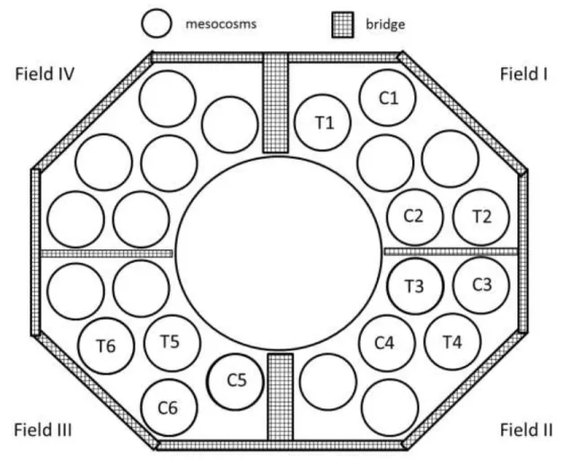
LakeLab, the depths of the enclosures vary between 17 and 20 m. Twelve enclosures were 90
randomly selected for the experiments from Fields I-III (Fig. 1). Prior to the experiment, water 91
exchange was performed in all mesocosms to ensure the possible highest similarity. The 92
thermocline was deepened by 2 m experimentally in 6 of 12 mesocosms; the other six mesocosms 93
served as controls. The water exchange and the alteration of the stratification was performed by 94
submerged pumps (SUPS 4-12-5, SPECK Pumpen Verkaufsgesellschaft GmbH, Neunkirchen am 95
Sand, Germany) transporting nearly 6 m3 h-1 of water via aluminium release rings. The graphical 96
design of the system is found in Fuchs et al. (2017). During the experiment surface water was 97
pumped down to a given depth only during daytime to allow the natural cooling over nights.
98
During the first month, rhythm of pumping activity was 8 h per day, then until the end of the 99
experiment it was increased to 12 h per day. In the control mesocosms, aluminium rings were 100
placed in the depth of the lake’s thermocline in order to affect equally all systems by pumping 101
activities. The depth of the release rings were moved 1 m down at 24 July, 25 July and 04 102
September to follow the natural thermocline depth in the lake.
103
Physical and chemical parameters (temperature, conductivity, pH, redox potential, oxygen 104
concentration, oxygen saturation and the photosynthetically available radiation - PAR) were 105
measured with YSI (Yellow Springs Instruments, OH, USA) and PAR sensors. These data were 106
recorded in half a meter increments from the surface (0.5 m) to the bottom in every hour.
107
Integrated water samples were taken on 25 June, 10 July, 23 July, 06 August, 20 August, and 11 108
September 2013 both from the epi- and hypolimnion using an integrated water sampler (IWS II, 109
Volume: 5L, Hydro-Bios, Kiel, Germany). Concentrations of TP, SRP, TN, NO2-
, NO3-
, NH4+
110
and SRSi were measured according to APHA (1998) in these samples. All inorganic N fractions 111
(NO2-
-N, NO3-
-N and NH4+
-N) were added for estimating dissolved inorganic nitrogen (DIN), 112
and nutrient ratio (DIN/SRP). Samples for phytoplankton analyses were taken on 25 June, 23 113
July, 20 August 2013. These samples were preserved in Lugol’s solution and were stored in a 114
dark at room temperature. Phytoplankton numbers were determined with the classical 115
methodology by Utermöhl (1958) and Lund et al. (1958). Altogether 400 settling units (cells, 116
filaments and colonies) were counted at minimum in each sample using an inverted microscope 117
(Zeiss Axiovert 100, Oberkochen, Germany). Volume of the cells was calculated by the most 118
similar geometric form according to Hillebrand et al. (1999), then biovolume was converted to 119
biomass using the 1 mm3L-1 = 1 mgL-1 conversion factor. Opticount cell counting software 120
(Opticount, 2008) was used to estimate the biomass. Phytoplankton species were sorted into 121
different functional groups (FG) according the classification of Reynolds et al. (2002) and 122
Padisák et al. (2009).
123
Analysis of variance using distance matrices was used to test how depth (epilimnion or 124
hypolimnion), month of the sampling (June, July, August) and treatment (control, treatment) 125
influence the community composition using function ADONIS in R software (R Core Team, 126
2015). Bray-Curtis dissimilarity was used for the distance matrix. Indicator species analysis 127
according to Dufrene and Legendre (1997) was run to identify characteristic taxa of depths, 128
months and treatments. INDVAL function was used by the labdsv package (Roberts, 2012) in R 129
environment.
130 131
Results 132
133
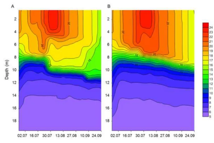
The alteration of the thermocline depth resulted in multiple changes in the stratification pattern:
134
the border between hypolimnion and metalimnion sank, and according to the temperature the 135
epilimnion had two parts. The temperature of upper part (from the surface until 4 meter) was 136
homogenous and the lower part had a small temperature decrease until metalimnion. The 137
temperature was rather smooth in the epilimnion of control mesocosms. The typical temperature 138
profile of the treatment and control mesocosms are shown in Fig. 2. Similar patterns were 139
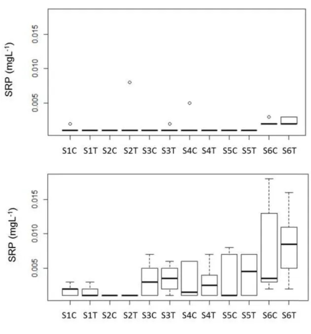
observed in the control and treatment mesocosms related to SRP values: at the beginning, the 140
amounts of SRP fall near to the detection limit in both in the epilimnion and hypolimnion, later 141
SRP in the epilimnion remained low during the whole experiment, but it increased in the 142
hypolimnion after mid-July. In spite of the similar pattern, the medians of SRP were higher in the 143
hypolimnion of treatment mesocosms compared to the controls (Fig. 3), however there were no 144
significant differences between the treatment and control mesocosms according to t-test analyses.
145
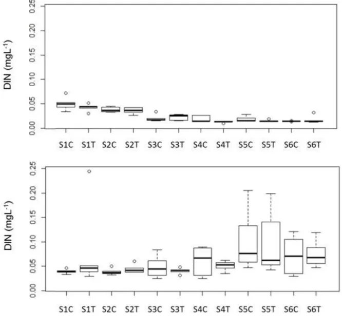
The DIN values were close to 0.05 mgL-1 at beginning of the experiment in the hypolimnion and 146
epilimnion as well, in both types of mesocosms (Fig. 4). Later, it decreased in the epilimnion and 147
increased in the hypolimnion both in the treatment and control mesocosms. The maximum level 148
of DIN/SRP (92) was calculated in a hypolimnetic sample at the beginning of September and the 149
lowest value (4) was calculated at the end of the experiment in several epilimnetic samples. In 150
general, the DIN/SRP values decreased in the epilimnion and alternated in the hypolimnion.
151
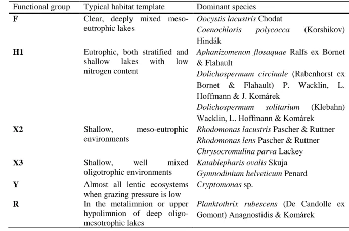
Altogether 78 samples were analysed and 130 taxa were found in these samples. Species 152
can be categorised in 21 functional groups of which F, H1, X2, X3, and Y were the most 153
frequently occurring FGs present in more than 90 % of the samples and R, H1 and Y were the 154
most dominant ones. The main representatives of the FG’s are shown in Table 1.
155
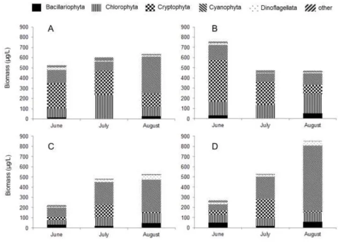
Cryptophytes were the most dominant phytoplankton group in the epilimnetic samples at 156
the beginning of the experiment (Fig. 5 A, C). Later this group strongly decreased in the control 157
mesocosms until the end of the experiment. Chlorophytes showed maximum abundance during 158
July in the epilimnetic samples of the treatment mesocosm, but reached maximum level during 159
August in the control enclosures. The biomass of cyanobacteria showed increasing pattern during 160
the experiment, and reached the highest amount during August as well.
161
Maximum abundance of cryptophytes was registered during July in the hypolimnion of 162
both types of mesocosms (Fig. 5 B, D). Biomass of dinoflagellates showed increasing pattern in 163
the treatment and control mesocosms as well. Similar amount of Chlorophytes were present in the 164
two types of mesocosms in the hypolimnion. Furthermore, cyanobacteria was the most dominant 165
taxonomic group reaching 59% contribution to total biomass in the treatment mesocosms and 166
75% in the control enclosures. Species belonging to the chrysophytes were observed in negligible 167
amounts. Diatoms occurred rarely in our experiment, although higher amounts were registered in 168
the hypolimnetic samples but remaining below 12% of the total biomass.
169
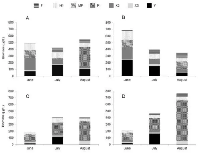
The changes of the seven most dominant functional groups are shown on Figure 6. At the 170
beginning, H1, X2 and Y coda dominated in the epilimnetic samples. The abundance of the latter 171
was higher in the epilimnion of control mesocosms, than in the treatment one (Fig. 6 A, C). At 172
the end of the experiment, decrease of the total biomass was observed in the control mesocosms, 173
but a slight increase was registered in the treatment enclosures. This difference was caused by 174
high amounts of Planktothrix rubescens (the only member of codon R), which started to increase 175
after July in the treatment enclosures. This species dominated in the hypolimnetic samples and 176
started to increase from the beginning of the experiment and became the most dominant by 177
August. That time, nearly 70% of the total biomass belonged to this species (functional group) in 178
the control mesocosms and reached 51% in the treatment enclosures in the hypolimnion.
179
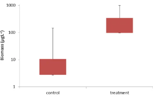
However, in the epilimnia P. rubescens reached 8% (32.9±62.2) in the control mesocosms and 180
44% (342.3±381.6) in the treatment enclosures (Fig. 7). This difference was significant according 181
to Wilcoxon test: W=2, p=0.03175.
182
Phacotus lenticularis (Ehrenberg) Deising was the only member of XPh codon, and did not 183
belong to the frequently occurring functional groups. However, during July it became the 184
dominant member of the phytoplankton community in mesocosm T6; while remaining low in 185
other mesocosms (not shown) and nearly disappeared from T6 during August. Thus this codon 186
caused the highest uncertainty during the experiment.
187
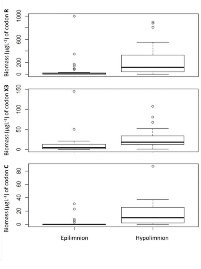
ADONIS revealed that the depths (epi-, or hypolimnion), months and treatment 188
individually, further the interaction of months and depths affect significantly the phytoplankton 189
community composition of mesocosms (Table 2). INDVAL analyses were performed to 190
investigate, which functional groups indicate the different categories of months, depths and 191
treatment (Table 3). Six functional groups (X2, L0, X1, Y, F and H1) were indicators of 192
epilimnetic samples and 3 coda (R, X3 and C) were indicators of hypolimnetic samples (Fig. 8).
193
Interestingly, INDVAL did not find any indicator codon for treatment or control mesocosms.
194
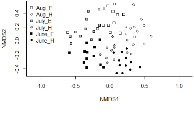
NMDS analyses (Fig. 9) were carried out to visualize differences between samples 195
belonging to different months, treatment and depths suggested by ADONIS analyses. Epilimnetic 196
and hypolimnetic samples are separated according mainly to the vertical axis, other samples from 197
different months differentiated based mainly on the horizontal axis.
198 199
Discussion 200
201
The heat-balance of lakes is determined basically by meteorological forcing at the air-water 202
interface, therefore, it is possible to raise general predictions for changes of the thermal 203
characteristics of lakes in relation to climate change. However, other features such as 204
morphometry, residence time of water, optical properties and landscape setting can have a major 205
effect on the thermal characteristic of lakes (Arvola et al., 2010). For this reason, lakes respond 206
individually to the effect of climate change concerning changes of stratification pattern and very 207
likely to numerous other hydrological and chemical changes as well. For example, both shrinking 208
and deepening of thermoclines were predicted and observed in a number of studies. Model 209
predictions for four Finish lakes suggested thermocline deepening in three cases and a shallower 210
thermocline in one case (Elo et al., 1998). In North-temperate lakes in Wisconsin (USA), 211
analyses of 10-year thermal records predicted changes in thermocline depth ranging from 3.5 m 212
deeper to 4.0 m shallower compared to the average depth (DeStasio et al., 1996). Thermocline 213
deepening was observed during long term studies (1970-1990) in Canadian boreal lakes by 214
Schindler et al. (1996) and it was explained by three reasons: (i) increasing wind velocities, (ii) 215
increasing effects of wind, because of decreasing number of trees in the area, however, the most 216
important reason was (iii) the rising temperature in sub-thermocline water layers caused by 217
increasing transparency of epilimnetic water. Fee et al. (1996) got similar outcome and the 218
authors emphasised that the increasing transparency is an important factor especially in case of 219
small lakes (<500 ha). The increase in Secchi-depths was the consequence of decreasing DOC 220
level because of the less precipitation runoff caused by longer periods of droughts.
221
The general findings of numerous studies is that warmer air temperatures result in warmer 222
surface water temperature and this layer of warmer and lighter water weakens wind induced 223
mixing, thus shallower and warmer epilimnia are predicted in the future (Robertson and 224
Ragotzkie, 1990; King et al., 1997; Vincent, 2009; De Senerpont Domis et al., 2013). Coats et al.
225
(2006) analysed the thermal structure of Lake Tahoe (USA) from 1970 to 2002 and observed a 226
strong decrease of depth of the October thermocline, but the reasons remained unrevealed. Straile 227
et al. (2003) and Livingstone (2003) analysed long dataset from deep European lakes (Lake 228
Constance and Lake Zürich) and they found increasing epilimnetic temperatures like in most of 229
the studied lakes around the globe, although these two studies did not observe clear changes 230
related to thermocline depth.
231
Thus it is possible to draw an important lesson from these examples, namely that we must 232
be cautious with general statements related to lake responses to climate change, because even 233
quite similar lakes can react at different ways to changing climatic conditions.
234
Either the thermocline depth of Lake Stechlin will decrease or increase in the future, it is 235
likely to result in changes in overall phytoplankton biomass and taxonomic composition, because 236
mixing depth is a key factor determining light availability and sedimentation losses (Reynolds, 237
1984; Visser et al., 1996).
238
In our experiment, the thermocline of treated mesocosms was deepened by 2 meters 239
compared to the control mesocosms and small, but strongly significant (P<0.001) differences 240
were observed between the phytoplankton community composition of the treated and control 241
enclosures. The observed differences confirm the prominent importance of position of the mixing 242
depth. The most obvious difference between the control and treatment mesocosms is the high 243
abundance of Planktothrix rubescens in the epilimnion of treatment- and in the hypolimnion of 244
control enclosures. Moreover, the amounts of chlorophytes were higher in the epilimnion of 245
control mesocosms during the last month, as a consequence of the considerable abundance of F 246
and MP coda.
247
Similar, but more spectacular results were found by Cantin et al. (2011) in an experiment of 248
thermocline deepening, however at a whole basin scale not in mesocosms. The authors could 249
demonstrate an important shift in the structure of the phytoplankton community towards 250
dominance of chlorophytes in the epilimnion in response to thermocline deepening. In our 251
experiment we did not observe this phenomenon, although green algae belonging to codon F, 252
such as Oocystis lacustris Chodat, frequently occurred in epilimnetic samples, and reached higher 253
biomass in the control mesocosms.
254
Ptacnik et al. (2003) analysed the phytoplankton community changes in a gradient of 255
mixing depths in a mesocosm experiment. High biomass of diatoms was observed in this 256
experiment even at low mixing depth and it was explained by the fast growth rates of diatoms 257
under sufficient supply of available silica. Our experiment cannot support the increase of 258
diatoms, because this group never exceeded a 12% contribution to the total biomass, though in 259
more than 80% of the samples the SRSi concentration was higher than 0.1 mgL-1 but none of 260
them was higher than 0.5 mgL-1. According to Reynolds (2006) silica concentration below 0.5 261
mgL-1 begins to interfere the growth of diatoms, but the growth-limiting threshold is 0.1 mgL-1 or 262
less in most lacustrine environments. Sommer (1988) reviewed a number of experimental and 263
field observations and concluded that the limitation is strongly species-specific and ranges 264
between 0.9 μM Si (~0.023 mgL-1) and 20 μM Si (~0.5 mgL-1). Others indicate 0.5 mgL-1 as 265
limitation threshold for Asterionella formosa Hassall, (Lund, 1950; Vaccari et al., 2006), which 266
was the most dominant diatom species during our experiment.
267
At beginning of the experiment cryptophytes were the dominant taxonomic group in all the 268
epilimnetic samples in the treatment and control mesocosms as well, which can be explained by 269
the effect of pumping activity which can be considered as a kind of disturbance. This group can 270
be prominent in post-stratification community or can peaks after disturbances such as 271
precipitation periods or wind activity (Reynolds and Reynolds, 1985; Bicudo et al., 2009). During 272
July cryptophytes increased in the hypolimnetic samples and decreased in the epilimnion. The 273
epilimnetic decline could be related to the increasing zooplankton grazing and may the deepened 274
thermocline favoured to cryptophytes to increase their biomass in the hypolimnion. Cryptophytes 275
can have competitive advantage there, because in case of deeper thermocline the nutrient-rich 276
hypolimnion has lower light levels, which they can utilize with special pigments such as carotene 277
or phycoerythrin (Gervais, 1997) or they can compensate with mixotrophic strategy (Cantin et al., 278
2011). However, the reason of the cryptophytes increase was most probably their disturbance 279
tolerance.
280
Planktothrix rubescens is an important member of the phytoplankton community of Lake 281
Stechlin for a long time (Krieger, 1927). The abundance of this species is commonly low, 282
however, if the circumstances are appropriate it can become the dominant taxon in the lake, such 283
as in 1998 (Padisák et al., 2003) or in the year of this study (2013) (Selmeczy et al., 2016).
284
During these periods, this species can be classified as an “ecosystem engineer”, because it can 285
strongly modify the annual phytoplankton succession of the lake (Padisák et al., 2010).
286
Planktothrix rubescens is typical a deep-chlorophyll maximum (DCM) forming cyanobacterium 287
in the metalimnion or in the upper hypolimnion in deep lakes (Micheletti et al., 1998; Camacho, 288
2006), thus the depth of the thermocline is very likely crucial for this species. The euphotic depth 289
of Lake Stechlin extends to the upper 20-25 meter and the thermocline develops around 8 meter 290
below the surface during the stratified period, thus there is a more or less 10-15 meter thick water 291
layer available for DCM formation. If the thermocline will lower because of the climate change 292
by two or even more meters, still there is “enough space” for DCM forming phytoplankton 293
species. Thus we can conclude that the thermocline deepening is not likely to affect the 294
development of DCM by Planktothrix rubescens. However, other species such as 295
Aphanizomenon flosaquae Ralfs ex Bornet & Flahault, or more frequently Cyanobium sp. can 296
form DCM in Lake Stechlin as well. According to our experience these species are forming DCM 297
in the middle of the thermocline (Padisák, 2003; Selmeczy et al., 2016) mainly spatially separated 298
from the population of Planktothrix rubescens. However, if the thermocline depth will increase, 299
the amount of available light will decrease, which basically influences the community of DCM 300
forming species. Consequently, P. rubescens may outcompete the above mentioned species, if the 301
thermocline depth increases until a certain point, because P. rubescens, can utilize low light 302
levels much more effectively than either Aphanizomenon flosaquae or Cyanobium sp.
303
Additionally, Planktothrix rubescens can produce cyanotoxins in Lake Stechlin (Dadheech et al., 304
2014), which justifies the necessity of regular monitoring of the species. In spite of the typical 305
characteristic of this species, according to our experiment P. rubescens can be a good competitor 306
in the epilimnion as well, because during August it became the dominant species in the 307
epilimnion of treatment mesocosms. This phenomenon is interesting, because it was rarely 308
described (e.g. Anneville et al., 2014) that higher or at least comparable biomass of P. rubescens 309
occurred in the epilimnion, as in the meta,- or upper hypolimnion in case of deep lakes. A 310
possible explanation is that the lower part of epilimnion offered good conditions for P. rubescens.
311
This zone had a slightly lower temperature compared to the same depths of the control 312
mesocosms, however, because of the lack of samples from different depth increments, it is not 313
possible to confirm this hypotheses.
314
IndVal analyses did not detect any functional group which would be specific to the 315
phytoplankton assemblage of either the treatment or the control mesocosms, however statistically 316
significant differences were registered between them. Thus, the differences between the two 317
communities related to numerous smaller or bigger differences in the proportion of different 318
functional groups, instead of emerging one or few groups, which are present just in one type of 319
mesocosms. However, on species level, significant difference was found related to the biomass of 320
P. rubescens, but only in the epilimnetic samples during August. This was the most remarkable 321
difference, which was registered during end of the experiment and this can be explained by the 322
high resilience of the community. Additionally, according to IndVal analyses the temporal 323
changes (different months) and different depths have a stronger effect on the community, than the 324
altered thermocline.
325
As a conclusion, the artificial deepening of the thermocline led to small, but significant 326
changes in the epilimnetic phytoplankton community: higher level of biomass of Planktothix 327
rubescens (codon R) and lower amounts of coda F and MP were registered after the treatment.
328
Additionally, P. rubescens was the dominant member of the phytoplankton community in the 329
treatment mesocosms, however it is not a clear confirmation about the proliferation of 330
cyanobacteria related to a deepened thermocline, because in 2013, when the study was 331
conducted, P. rubescens were present with high biomass during the whole vegetation period, 332
similarly to 1998 (Padisák et al., 2010), therefore presumably the summer phytoplankton 333
assemblage was considerably affected by P. rubescens.
334 335
Acknowledgement 336
337
We are grateful to the entire team of the TemBi project for the planning, preparation and 338
conduction of the experiment: U. Beyer, C. Engelhardt, A. Fuchs, M. O. Gessner, H.-P. Grossart, 339
T. Hornick, J. Hüpeden, E. Huth, C. Kasprzak, P. Kasprzak, G. Kirillin, M. Lentz, E. Mach, U.
340
Mallok, G. Mohr, M. Monaghan, M. Papke, R. Rossberg, M. Sachtleben, J. Sareyka, M. Soeter, 341
C. Wurzbacher and E. Zwirnmann. We thank Andrea Fuchs for her ideas related to statistical 342
analyses. Furthermore, we thank the anonymous reviewers who helped to improve the 343
manuscript. The project “TemBi - Climate driven changes in biodiversity of microbiota” is 344
granted by the Leibniz society (SAW-2011-IGB-2). Partial support was provided by the 345
Hungarian National Research, Development and Innovation Office (NKFIH K-120595).
346 347
References 348
349
APHA-American Public Health Association, 1998. Standard Methods for the Examination of 350
Water and Wastewater, 20th edn. United Book Press Inc, Baltimore, MD.
351
Arvola, L., G. George, D. M. Livingstone, M. Järvinen, T. Blenckner, M. T. Dokulil, E. Jennings, 352
C. N. Aonghusa, P. Nõges, T. Nõges & G. A. Weyhenmeyer, 2010. The Impact of the 353
Changing Climate on the Thermal Characteristics of Lakes. In George, G. (ed) The 354
Impact of Climate Change on European Lakes. Aquatic Ecology Series, vol 4. Springer 355
Netherlands, 85-101.
356
Bauchrowitz, M., 2012. The LakeLab – A new experimental platform to study impacts of global 357
climate change on lakes. SIL News 60:10-12.
358
Behrenfeld, M. J., R. T. O’Malley, D. A. Siegel, C. R. McClain, J. L. Sarmiento, G. C. Feldman, 359
A. J. Milligan, P. G. Falkowski, R. M. Letelier & E. S. Boss, 2006. Climate-driven trends 360
in contemporary ocean productivity. Nature 444:752-755.
361
Bicudo, C. E. d. M., C. Ferragut & M. R. Massagardi, 2009. Cryptophyceae population dynamics 362
in an oligo-mesotrophic reservoir (Ninféias pond) in São Paulo, southeast Brazil. Hoehnea 363
36:99-111.
364
Camacho, A., 2006. On the occurrence and ecological features of deep chlorophyll maxima 365
(DCM) in Spanish stratified lakes. Limnetica 25:453-478.
366
Cantin, A., B. E. Beisner, J. M. Gunn, Y. T. Prairie & J. G. Winter, 2011. Effects of thermocline 367
deepening on lake plankton communities. Canadian Journal of Fisheries and Aquatic 368
Sciences 68:260-276.
369
Carey, C. C., B. W. Ibelings, E. P. Hoffmann, D. P. Hamilton & J. D. Brookes, 2012. Eco- 370
physiological adaptations that favour freshwater cyanobacteria in a changing climate.
371
Water Research 46:1394-1407.
372
Casper, S. J., 1985. Lake Stechlin. A temperate oligotrophic lake. Dr. W. Junk Publishers, 373
Dordrecht, Netherlands.
374
Coats, R., J. Perez-Losada, G. Schladow, R. Richards & C. Goldman, 2006. The warming of lake 375
Tahoe. Climatic Change 76:121-148.
376
Dadheech, P. K., G. B. Selmeczy, G. Vasas, J. Padisák, W. Arp, K. Tapolczai, P. Casper & L.
377
Krienitz, 2014. Presence of potential toxin-producing cyanobacteria in an oligo- 378
mesotrophic lake in Baltic Lake District, Germany: An ecological, genetic and 379
toxicological survey. Toxins 6:2912-2931.
380
De Senerpont Domis, L. N., J. J. Elser, A. S. Gsell, V. L. M. Huszar, B. W. Ibelings, E. Jeppesen, 381
S. Kosten, W. M. Mooij, F. Roland, U. Sommer, E. Van Donk, M. Winder & M. Lürling, 382
2013. Plankton dynamics under different climatic conditions in space and time.
383
Freshwater Biology 58:463-482.
384
DeStasio, B. T., D. K. Hill, J. M. Kleinhans, N. P. Nibbelink & J. J. Magnuson, 1996. Potential 385
effects of global climate change on small north-temperate lakes: Physics, fish, and 386
plankton. Limnology and Oceanography 41:1136-1149.
387
Dufrene, M. & P. Legendre, 1997. Species assemblages and indicator species: the need for a 388
flexible asymmetrical approach. Ecological Monographs 67:345-366.
389
Ehling-Schulz, M. & S. Scherer, 1999. UV protection in cyanobacteria. European Journal of 390
Phycology 34:329-338.
391
Elo, A.-R., T. Huttula, A. Peltonen & J. Virta, 1998. The effects of climate change on the 392
temperature conditions of lakes. Boreal Environment Research 3:137-150.
393
Fee, E. J., R. E. Hecky, S. E. M. Kasian & D. R. Cruikshank, 1996. Effects of lake size, water 394
clarity, and climatic variability on mixing depths in Canadian Shield lakes. Limnology 395
and Oceanography 41:912-920.
396
Findlay, D. L., S. E. M. Kasian, M. P. Stainton, K. Beaty & M. Lyng, 2001. Climatic influences 397
on algal populations of boreal forest lakes in the experimental lakes area. Limnology and 398
Oceanography 46:1784-1793.
399
Fuchs, A., J. Klier, F. Pinto, G. B. Selmeczy, B. Szabó, J. Padisák, K. Jürgens & P. Casper, 2017.
400
Effects of artificial thermocline deepening on sedimentation rates and microbial processes 401
in the sediment. Hydrobiologia, DOI 10.1007/s10750-017-3202-7.
402
Gerten, D. & R. Adrian, 2002. Responses of lake temperatures to diverse North Atlantic 403
Oscillation indices. In Wetzel, R. G. (ed) International Association of Theoretical and 404
Applied Limnology Proceedings. E Schweizerbart’sche Verlagsbuchhandlung, Stuttgart, 405
1593-1596.
406
Gervais, F., 1997. Diel vertical migration of Cryptomonas and Chromatium in the deep 407
chlorophyll maximum of a eutrophic lake. Journal of Plankton Research 19:533-550.
408
Hillebrand, H., C.-D. Dürselen, D. Kirschtel, U. Pollingher & T. Zohary, 1999. Biovolume 409
calculation for pelagic and benthic microalgae. Journal of Phycology 35:403-424.
410
Huisman, J., J. Sharples, J. M. Stroom, P. M. Visser, W. E. A. Kardinaal, J. M. H. Verspagen &
411
B. Sommeijer, 2004. Changes in turbulent mixing shift competition for light between 412
phytoplankton species. Ecology 85:2960-2970.
413
IPCC, 2007. Summary for policymakers. In: Pachauri, R. K. & A. Reisinger (eds) Climate 414
Change 2007: Synthesis Report. Geneva, Switzerland.
415
IPCC, 2013. Climate Change 2013: The Physical Science Basis. Contribution of Working Group 416
I to the Fifth Assessment Report of the Intergovernmental Panel on Climate Change. In:
417
Stocker, T. F., et al. (eds). Cambridge University Press, Cambrigde, United Kingdom and 418
New York, USA.
419
King, J. R., B. J. Shuter & A. P. Zimmerman, 1997. The response of the thermal stratification of 420
South Bay (Lake Huron) to climatic variability. Canadian Journal of Fisheries and 421
Aquatic Sciences 54:1873-1882.
422
Krieger, W., 1927. Die Gattung Centronella Voigt. Berichte der Deutschen Botanischen 423
Gesellschaft 45:281-290.
424
Livingstone, D. M., 2003. Impact of secular climate change on the thermal structure of a large 425
temperate central European lake. Climatic Change 57:205-225.
426
Lund, J. W. G., 1950. Studies on Asterionella formosa Hass: II. Nutrient Depletion and the 427
Spring Maximum. Journal of Ecology 38:15-35.
428
Lund, J. W. G., C. Kipling & E. D. Le Cren, 1958. The inverted microscope method of estimating 429
algal numbers and the statistical basis of estimations by counting. Hydrobiologia 11:143- 430
170.
431
Medeiros, L. D., A. Mattos, M. Lurling & V. Becker, 2015. In the future blue-green or brown?
432
The effects of extreme events on phytoplankton dynamics in a semi-arid man-made lake.
433
Aquatic Ecology 49:293-307.
434
Micheletti, S., F. Schanz & A. E. Walsby, 1998. The daily integral of photosynthesis by 435
Planktothrix rubescens during summer stratification and autumnal mixing in Lake Zürich.
436
New Phytologist 139:233-246.
437
OPTICOUNT, 2008. http://science.do-mix.de/software_opticount.php.
438
Padisák, J., O. L. Crossetti & L. Naselli-Flores, 2009. Use and misuse in the application of the 439
phytoplankton functional classification: a critical review with updates. Hydrobiologia 440
621:1-19.
441
Padisák, J., É. Hajnal, L. Krienitz, J. Lakner & V. Üveges, 2010. Rarity, ecological memory, rate 442
of floral change in phytoplankton – and the mystery of the Red Cock. Hydrobiologia 443
653:45-64.
444
Padisák, J., W. Scheffler, P. Kasprzak, R. Koschel & L. Krienitz, 2003. Interannual variability in 445
the phytoplankton compostion of Lake Stechlin (1994-2000). Archiv für Hydrobiologie, 446
Special Issues, Advances in Limnology 58:101-133.
447
Ptacnik, R., S. Diehl & S. Berger, 2003. Performance of sinking and nonsinking phytoplankton 448
taxa in a gradient of mixing depths. Limnology and Oceanography 48:1903-1912.
449
R Core Team, 2015. A language and environment for statistical computing. http://www.R- 450
project.org/.
451
Reynolds, C. S., 1984. The ecology of freshwater phytoplankton. Cambridge University Press.
452
Reynolds, C. S., 2006. Ecology of phytoplankton. Cambridge University Press, Cambridge.
453
Reynolds, C. S., V. Huszar, C. Kruk, L. Naselli-Flores & S. Melo, 2002. Towards a functional 454
classification of the freshwater phytoplankton. Journal of Plankton Research 24:417-428.
455
Reynolds, C. S. & J. B. Reynolds, 1985. The atypical seasonality of phytoplankton in Crose 456
Mere, 1972: an independent test of the hypothesis that variability in the physical 457
environment regulates community dynamics and structure. British Phycological Journal 458
20:227-242.
459
Roberts, D. W., 2012. labdsv: ordination and multivariate analysis for ecology. http://CRAN.R- 460
project.org/package=labdsv.
461
Robertson, D. M. & R. A. Ragotzkie, 1990. Changes in the thermal structure of moderate to large 462
sized lakes in response to changes in air temperature. Aquatic Sciences 52:360-380.
463
Salmaso, N., A. Boscaini, C. Capelli, L. Cerasino, M. Milan, S. Putelli & M. Tolotti, 2015.
464
Historical colonization patterns of Dolichospermum lemmermannii (Cyanobacteria) in a 465
deep lake south of the Alps. Advances in Oceanography and Limnology 6:35-45.
466
Schindler, D. W., S. E. Bayley, B. R. Parker, K. G. Beaty, D. R. Cruikshank, E. J. Fee, E. U.
467
Schindler & M. P. Stainton, 1996. The effects of climatic warming on the properties of 468
boreal lakes and streams at the Experimental Lakes Area, northwestern Ontario.
469
Limnology and Oceanography 41:1004-1017.
470
Selmeczy, G. B., K. Tapolczai, P. Casper, L. Krienitz & J. Padisák, 2016. Spatial- and niche 471
segregation of DCM-forming cyanobacteria in Lake Stechlin (Germany) Hydrobiologia 472
764:229-240.
473
Sommer, U., 1988. Growth and survival strategies of planktonic diatoms. In Sandgren, C. D. (ed) 474
Growth and Reproductive Strategies of Freshwater Phytoplankton. Cambrigde University 475
Press, Cambridge 227-260.
476
Straile, D., K. D. Jöhnk & H. Rossknecht, 2003. Complex effects of winter warming on the 477
physicochemical characteristics of a deep lake. Limnology and Oceanography 48:1432- 478
1438.
479
Sukenik, A., A. Quesada & N. Salmaso, 2015. Global expansion of toxic and non-toxic 480
cyanobacteria: effect on ecosystem funtioning. Biodiversity and Conservation 24:889- 481
908.
482
Turner, J. S., 1979. Buoyancy effetcs in fluids. Cambridge University Press, Cambridge.
483
Utermöhl, H., 1958. Zur Vervollkommnung der quantitativen Phytoplankton-Methodik.
484
Mitteilungen der internationalen Vereinigung für theoretische und angewandte 485
Limnologie 9:1-38.
486
Üveges, V., K. Tapolczai, L. Krienitz & J. Padisák, 2012. Photosynthetic characteristics and 487
physiological plasticity of an Aphanizomenon flos-aquae (Cyanobacteria, Nostocaceae) 488
winter bloom in a deep oligo-mesotrophic lake (Lake Stechlin, Germany). Hydrobiologia 489
698:263-272.
490
Vaccari, D. A., P. F. Strom & J. E. Alleman, 2006. Environmental biology for engineers and 491
scientists. John Wiley & Sons Inc., Hoboken, New Jersey.
492
Vincent, W. F., 2009. Effects of climate change on lakes. In Likens, G. E. (ed) Biogeochemistry 493
of inland waters. Elsevier, 611-616.
494
Visser, P. M., L. Massaut, J. Huisman & L. R. Mur, 1996. Sedimentation losses of Scendesmus in 495
relation to mixing depth. Archiv für Hydrobiologie 136:276-277.
496
Winder, M., J. E. Reuter & S. G. Schladow, 2009. Lake warming favours small-sized planktonic 497
diatom species. Proceedings of the Royal Society B 276:427-435.
498
Winder, M. & U. Sommer, 2012. Phytoplankton response to a changing climate. Hydrobiologia 499
698:5-16.
500 501
502
503
Fig. 1 Lake Lab platform with the experimental design, C1, C2, C3, C4, C5, C6 indicate control 504
mesocosms and T1, T2, T3, T4, T5, T6 indicate treated mesocosms 505
506
507
508
Fig. 2 Typical temperature profiles of treatment (A) and control (B) mesocosms established in 509
Lake Stechlin between 25 June 2013 and 24 September 2013 510
511
512
513
Fig. 3 Boxplots of SRP values during the experiment in the epilimnion (upper panel) and in the 514
hypolimnion (lower panel), S1: 29 May, S2: 25 June, S3: 10 July, S4: 23 July, S5: 06 August, S6:
515
20 August; C indicates control, T indicates treatment mesocosms 516
517
518 519
Fig. 4 Boxplots of DIN values during the experiment in the epilimnion (upper panel) and in the 520
hypolimnion (lower panel), S1: 29 May, S2: 25 June, S3: 10 July, S4: 23 July, S5: 06 August, S6:
521
20 August; C indicates control, T indicates treatment mesocosms 522
523
524 525
Fig. 5 Average biomass of the different taxonomical groups during the experiment (A:
526
Epilimnion of treatment mesocosms, B: Hypolimnion of treatment mesocosms, C: Epilimnion of 527
control mesocosms, D: Hypolimnion of control mesocosms) 528
529
530 531
Fig. 6 Average biomass of the most dominant functional groups during the experiment (A:
532
Epilimnion of treatment mesocosms, B: Hypolimnion of treatment mesocosms, C: Epilimnion of 533
control mesocosms, D: Hypolimnion of control mesocosms) 534
535
536 537
Fig. 7 Boxplots of biomass (μgL-1) of Planktothrix rubescens in epilimnion during August 538
539
540 541
Fig. 8 Boxplots of biomass (μgL-1) of coda C, X3 and R in epilimnetic and hypolimnetic samples 542
543
544 545
Fig. 9 NMDS ordination diagram based on the functional group composition of the samples. E=
546
Epilimnetic samples, H=Hypolimnetic samples 547
548
Table 1 Most important representatives of the main functional groups with their typical habitat 549
template according to Padisák et al. (2009) 550
Functional group Typical habitat template Dominant species
F Clear, deeply mixed meso-
eutrophic lakes
Oocystis lacustris Chodat
Coenochloris polycocca (Korshikov) Hindák
H1 Eutrophic, both stratified and shallow lakes with low nitrogen content
Aphanizomenon flosaquae Ralfs ex Bornet
& Flahault
Dolichospermum circinale (Rabenhorst ex Bornet & Flahault) P. Wacklin, L.
Hoffmann & J. Komárek
Dolichospermum solitarium (Klebahn) Wacklin, L. Hoffmann & Komárek
X2 Shallow, meso-eutrophic
environments
Rhodomonas lacustris Pascher & Ruttner Rhodomonas lens Pascher & Ruttner Chrysocromulina parva Lackey
X3 Shallow, well mixed
oligotrophic environments
Katablepharis ovalis Skuja Gymnodinium helveticum Penard Y Almost all lentic ecosystems
when grazing pressure is low
Cryptomonas sp.
R In the metalimnion or upper hypolimnion of deep oligo- mesotrophic lakes
Planktothrix rubescens (De Candolle ex Gomont) Anagnostidis & Komárek
551 552
Table 2 Summary of analyses of variance using distance matrices (ADONIS) testing the 553
individual and joint effects of month, treatment and depth on community composition.
554
Significant factors are highlighted in bold.
555
Factors Df SS MS F R2 P
Month 2 3.8095 1.9047 14.0068 0.2307 0.001
Treatment 1 0.2225 0.2225 1.6361 0.0135 0.001
Depth 1 2.7321 2.7321 20.0906 0.1654 0.001
Month: treatment 2 0.2306 0.1153 0.8478 0.0140 0.590
Month: depth 2 0.8788 0.4394 3.2312 0.0532 0.002
Treatment: depth 1 0.1351 0.1351 0.9931 0.0082 0.412
Month: treatment: depth 2 0.3467 0.1734 1.2748 0.0210 0.238
Residuals 60 8.1593 0.1360 0.4941
Total 71 16.5146 1.0000
556
Table 3 Summary of IndVal analyses 557
558 Codon Indication Indicator value P
X2 Epilimnion 0.81 0.001
L0 Epilimnion 0.81 0.001
X1 Epilimnion 0.71 0.004
Y Epilimnion 0.70 0.004
F Epilimnion 0.67 0.041
H1 Epilimnion 0.63 0.039
R Hypolimnion 0.76 0.001
X3 Hypolimnion 0.70 0.002
C Hypolimnion 0.69 0.001
MP June 0.62 0.001
X2 June 0.56 0.001
C June 0.39 0.009
Y July 0.52 0.001
XPh July 0.52 0.007
A August 0.76 0.001
R August 0.72 0.001
J August 0.62 0.009
P August 0.56 0.001
L0 August 0.52 0.020
F August 0.52 0.031