Research Article
The Settlement Structure Is Reflected in Personal
Investments: Distance-Dependent Network Modularity-Based Measurement of Regional Attractiveness
Laszlo Gadar,
1,2Zsolt T. Kosztyan,
1,3and Janos Abonyi
41MTA-PE Budapest Ranking Research Group, University of Pannonia, Veszpr´em, Hungary
2Innopod Solutions Kft., Budapest, Hungary
3Department of Quantitative Methods, University of Pannonia, Veszpr´em, Hungary
4MTA-PE “Lendulet” Complex Systems Monitoring Research Group, University of Pannonia, Veszpr´em, Hungary
Correspondence should be addressed to Janos Abonyi; janos@abonyilab.com
Received 10 August 2018; Revised 24 October 2018; Accepted 8 November 2018; Published 5 December 2018
Academic Editor: Pasquale De Meo
Copyright © 2018 Laszlo Gadar et al. This is an open access article distributed under the Creative Commons Attribution License, which permits unrestricted use, distribution, and reproduction in any medium, provided the original work is properly cited.
How are ownership relationships distributed in the geographical space? Is physical proximity a significant factor in investment decisions? What is the impact of the capital city? How can the structure of investment patterns characterize the attractiveness and development of economic regions? To explore these issues, we analyze the network of company ownership in Hungary and determine how are connections are distributed in geographical space. Based on the calculation of the internal and external linking probabilities, we propose several measures to evaluate the attractiveness of towns and geographic regions. Community detection based on several null models indicates that modules of the network coincide with administrative regions, in which Budapest is the absolute centre, and where county centres function as hubs. Gravity model-based modularity analysis highlights that, besides the strong attraction of Budapest, geographical distance has a significant influence over the frequency of connections and the target nodes play the most significant role in link formation, which confirms that the analysis of the directed company-ownership network gives a good indication of regional attractiveness.
1. Introduction
Mining valuable information from social networks is a hard problem due to its dynamic nature [1, 2], complex structure [3, 4], and multidimensionality [5]. This paper deals with the structural issues as it tries to evaluate regional attrac- tiveness based on a set of goal-oriented null models identi- fied to describe the geographical distributions of company- ownership relations.
Complex multivariate socioeconomic data is widely used to monitor regional policy [6, 7]. As the usage of a dif- ferent set of variables results in various rankings, the def- inition and selection of socioeconomic variables are the key issue in these applications. The drawback of these indicator-based approaches is that although economic behav- ior is socially constructed and embedded in networks of interpersonal relations [8] and strong related to location
[9], the network structure of the economy is neglect- ed.
This paper adds a viewpoint to regional studies based on the analysis of how the network of personal investments and the founding of companies relate to the settlement hierarchy.
We assume that the socially embedded economy must have a network-based imprint in the company-ownership network which is a good indication of regional attractiveness.
Attractiveness is meaningful in preferential attachment networks, where the likelihood of a new connection is proportional to degree [10] and fitness [11] of the node. These models were generalized to handle initial attractiveness [12]
and latecomer nodes with a higher degree of fitness [11, 13].
It is important to note that these models generate power- law (degree) distributions that are similar to the distribution of socioeconomic variables of settlements indicating that preferential attachment is a process that can be used to
Volume 2018, Article ID 1306704, 16 pages https://doi.org/10.1155/2018/1306704
describe city grow [14–18]. In the case of geographically distributed networks, the likelihood of link formation is dependent on distance due to the cost of establishing con- nections and spatial constraints [19]. Connection costs also favor the formation of cliques and thus increase the clustering coefficient [20]. Space is important in social networks as most individuals connect with their spatial neighbors [20] to minimize their effort and maintain social ties [21]; e.g., the majority of our friends are in our spatial neighborhood [22].
The probability𝑃(𝑑)that distance𝑑separates two connected individuals is found to behave as 𝑃(𝑑) ∼ 𝑑−2 in terms of Belgian mobile phone data [23], or generally𝑃(𝑑) ∼ 𝑑−𝛿, as has been shown in the case of the social network of more than one million bloggers in the USA [24], in friendship network of Facebook users, and in email communication networks [25, 26].
The attractiveness of airports [27], countries for foreign investments [28], and touristic destinations [29] is evaluated based on socioeconomic variables. As many origins and destinations are present in these applications, the theory of bilateral trade flows accounts for the relative attractiveness of origin-destination pairs. The gravity model is one of the most successful empirical models in economics developed to describe such interactions across the space [30]. Almost 40 years ago, before the emergence of network science, Anderson suggested that as a force between two mass points, the number of trips from location𝑖to location𝑗, follows the (economic version) of the “Gravity” law, 𝐹(𝑑) ∼ 𝑃(𝑑) ∼ 𝐼𝛼1𝐼2𝛼𝑑−𝛿[31]. Nowadays, many complex networks embedded in space and spatial constraints may have an effect on their connectivity patterns such as trade markets [32], migration [33], traffic flow [34], and mobile communication [23] that can be successfully modeled by a gravity model, which was also successfully applied in link prediction [35].
We assume that regions that heavily rely on local resources consist of more internal connections that form modules in networks, so the modularity of the networks which reflect socioeconomic relationships can be used to measure regional attractiveness. The goal of modularity anal- ysis is to separate the network into groups of vertices that have fewer connections between them than inside the communi- ties [36]. In social network analysis, community detection is a basic step in understanding the structure, function, and semantics of networks [4]. Community analysis is performed in two separate phases: first, detection of meaningful commu- nity structure from a network, and second, evaluation of the appropriateness of the detected community structure [37].
Systematic deviations from a random configuration allow us to define a quantity called modularity, that is a measure of the quality of partitions. Newman-Girvan modularity considers only the degree of nodes as a null model which is equivalent to rewiring the network whilst preserving the degree sequence [38, 39]. This random model overlooks the spatial nature of the network; thus, modules are blind to spatial anomalies and fails to uncover modules determined by factors other than mere physical proximity [19], which is the reason why several distance-dependent null models have been proposed recently [19, 37, 40, 41].
Our goal is to use the tools of network community detection to evaluate the attractiveness of the elements of set- tlement hierarchies (towns, statistical subregions, counties, and regions) based on their modularities as well as internal and external connection densities. We study the internal connections of the ownership network through the point of view of Newman-Girvan, spatial and gravity-based null models. As the modularity is based on the difference between the actual and evaluated values of weight of edges, the real spatial network more accurately describes the null model, and the total modularity tends to be zero, so the modules highlight the hidden structural similarities. We developed a visualization technique to analyze these unknown effects on community structure which can explain the attractiveness of a settlement/region. Besides measuring the attractiveness, we utilize the Louvain community detection algorithm [42, 43]
to identify closely related regions. We examine the complete investment network of Hungarian companies to explore how the ownership connections are geographically distributed, what is the structure of the network, and what are the common connection directions, as well as how the extracted information is correlated to the settlement hierarchy. The studied database contains information about the owners and addresses of the companies. The results highlight the fact that distance dependence of the investment connections is more significant than was found in online social networks [22, 26, 44]. The analysis shows that the network is hierarchical and modular as well as shaped according to the settlement hierarchy, in which Budapest is the absolute center, and the centers of counties function as hubs.
The outline of this paper is as follows: Section 2.1 presents the company-ownership network. The metrics related to at- tractiveness are given in the Appendix. Section 2.2 describes the null models designed by us to measure modularity as well as handling physical proximity and presents how closely related regions can be explored based on the modularity- related merging of towns and subregions. The results and discussion are provided in Section 3.
2. Problem Formulation: Settlement Hierarchy and Community Structure in Personal Investment Patterns
2.1. Network Representation of Personal Investment Patterns.
The proposed methodology is based on the analysis of a directed investment network represented by an asymmetric biadjacency matrixA[𝑝,𝑐𝑜], whose elements are defined as
𝑎𝑖,𝑗[𝑝,𝑐𝑜]
={ {{
1 if the𝑖-th person owns the 𝑗-th company 0 otherwise.
(1)
As the addresses of the owners and their companies are known, connections between companies and their owners define ties between geographic locations.
According to the levels of the settlement hierarchy, a four- level study can be defined to describe how towns, regions,
LAU-21 LAU-22
3
1
NUTS-31
2
NUTS-32
NUTS-33 4
Owner Company
LAU-25
NUTS-21
3 6
LAU-27 LAU-28 4
LAU-2
LAU-2 LAU-2
LAU-1
LAU-1
LAU-1 LAU-1
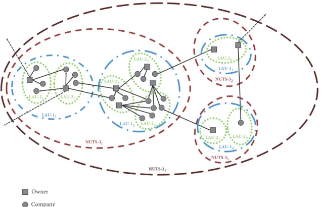
Figure 1: Company-ownership relations connect the elements of the settlement hierarchy (Settlement (LAU 2), statistical subregion (LAU 1), small-region (NUTS 3), and region (NUTS 2)).
or counties are connected through company ownerships (see Figure 1). Although companies also own shares in other companies, as we intended to study the attractiveness of economic regions based on personal investment decisions, we examined only companies that belong to individuals.
The levels of the settlement hierarchy[𝑙]are defined based on the nomenclature of territorial units for statistics classifi- cation (NUTS) and the two levels of local administrative units (LAUs):
𝑙
= {{ {{ {{ {{ {{ {{ {{ {
1 town/settlement - LAU2, formally NUTS5level 2 statistical sub-region - LAU1, formally NUTS4level 3 small regions/counties, NUTS3level
4 regions of regional policies, NUTS2level
(2)
(Please note that, for simplicity, the term “town” is used for all cities and villages.)
People and their companies are assigned to geographic regions by the A[𝑐𝑜,𝑙] and A[𝑝,𝑙] incidence matrices, whose elements are defined as follows:
(i)𝑎[𝑐𝑜,𝑙]𝑖,𝑗 with element one if the headquarter of the𝑖-th company is situated in the𝑗-th geographic region at the level𝑙of the settlement hierarchy,
(ii)𝑎[𝑝,𝑙]𝑖,𝑗 with element one if the 𝑖-th person is situated in the 𝑗-th geographic region at the level 𝑙 of the settlement hierarchy,
so the directed weighted network that defines the number of investment connections between the regions can be defined as
A[𝑙]= (A[𝑝,𝑙])𝑇×A[𝑝,𝑐𝑜]×A[𝑐𝑜,𝑙]. (3) Although companies may have many local divisions, the links between the towns are defined only by connecting the permanent addresses of the owners and the location of the headquarter. This arrangement results in a transparent and easily interpretable network as people and companies are assigned to only one location. The resultant network describes how investments unite the locations; e.g., the adjacency matrixA[1]defines the number of links between the towns, and the degrees of the nodes represent the number of incoming and outgoing investments to the𝑗-th and from the𝑖-th town, respectively:
𝑘[𝑙,𝑖𝑛]𝑗 = ∑
𝑖
𝑎[𝑙]𝑖,𝑗 (4)
𝑘[𝑙,𝑜𝑢𝑡]𝑖 = ∑
𝑗
𝑎[𝑙]𝑖,𝑗. (5) The total number of ownership relationships is equal to the sum of the edge weights of the networks:
𝐿 = ∑
𝑖
∑
𝑗
𝑎𝑖,𝑗[𝑙], ∀𝑙, (6) where𝑖and𝑗represent the indices of the geographic regions at the level𝑙of the settlement hierarchy.
It should be noted that as𝐿represents the total number of connections, its value is independent of at which hierarchy level the edge weights are summarised.
Similarly, the total number of companies and investors can be calculated by summing the number of companies and people at any hierarchy level, respectively:
𝑁[𝑐𝑜]= ∑
𝑗=1
𝑛[𝑙,𝑐𝑜]𝑗 ,
𝑁[𝑝]= ∑
𝑗=1
𝑛[𝑙,𝑝]𝑗 ,
∀𝑙,
(7)
where𝑗represents the index of the geographic regions at the level𝑙of the settlement hierarchy.
As people and companies are assigned only to one geo- graphical region with theA[𝑐𝑜,𝑙]andA[𝑝,𝑙]incidence matrices, the number of people and companies at the𝑗-th region of the [𝑙]-th level of the settlement hierarchy can be calculated as
𝑛[𝑙,𝑐𝑜]𝑗 = ∑
𝑖
𝑎[𝑐𝑜,𝑙]𝑖,𝑗 (8)
𝑛[𝑙,𝑝]𝑗 = ∑
𝑖
𝑎[𝑝,𝑙]𝑖,𝑗 . (9)
The number of internal and external links of the network and the analysis of the local densities can be used to measure the attractiveness of the regions (see the Appendix). The following main body of the paper focuses on models that can be used to explore the communities in the network.
2.2. Evaluation of the Community Structure in the Settle- ment Hierarchy. The key idea of the methodology is that geographical regions can be interpreted as nonoverlapping communities of investors and companies as they belong to exactly one region among the set of these regions on the𝑙-th level of the hierarchy,𝐶[𝑙]= {𝐶[𝑙]1 , 𝐶[𝑙]2 , . . . , 𝐶[𝑙]𝑙 , . . . , 𝐶[𝑙]𝑛𝑐,𝑛𝑘}.
From the view of a community, the external degree is the number of links that connect the 𝑖-th community to the rest of the network, while the internal degree is the number of links between companies and owners in the same community, in other words, at the same location at the 𝑙- th level of the hierarchy (for more details see Appendix A).
Recently, a wide variety of𝑓(𝐶)metrics have been proposed to evaluate the quality of communities on the basis of the connectivity of their nodes [37]. The following subsections will demonstrate how these metrics can be interpreted to evaluate the attractiveness of geographical regions.
2.2.1. Modularity of a Region and Level of a Settlement Hier- archy. Classical modularity optimization-based community detection methods utilize𝑓(𝐶)metrics that are based on the difference between the internal number of edges and their expected number [39, 45]:
𝑓 (𝐶) = (fraction of edges within communities)
− (expected fraction of such edges) . (10)
In the case of the proposed directed network, this differ- ence can be formulated as
𝑓 (𝐶[𝑙]) = 1 𝐿∑
𝑖,𝑗
(𝑎𝑖,𝑗[1]− 𝑝𝑖,𝑗[1]) 𝛿 (𝐶[𝑙]𝑖 , 𝐶[𝑙]𝑗 ) , (11)
where 𝑝[1]𝑖,𝑗 represents the number of estimated invest- ments proceeding from the 𝑖-th to the 𝑗-th town and 𝛿(𝐶[𝑙]𝑖 , 𝐶[𝑙]𝑗 )is the Kronecker delta function that is equal to one, if the𝑖-th and𝑗-th towns are assigned to the same region on the𝑙-th level of the hierarchy (e.g.,𝛿(𝐶[2]𝐴, 𝐶[2]𝐵 ) = 1when towns A and B are situated in the same statistical subregion).
The modularity of the partition𝐶[𝑙] can be calculated as the sum of the modularities of the𝐶[𝑙]𝑐 , 𝑐 = 1, . . . , 𝑛[𝑙]𝑐 commu- nities:
𝑀𝑐[𝑙]= 1
𝐿 ∑
(𝑖,𝑗)∈𝐶[𝑙]𝑐
(𝑎𝑖,𝑗[1]− 𝑝[1]𝑖,𝑗) . (12)
The value of the modularity𝑀𝑐[𝑙]of a cluster/region𝐶[𝑙]𝑐 can be positive, negative, or zero. Should it be equal to zero, the community has as many links as the null model predicts.
When the modularity is positive, then the𝐶[𝑙]𝑐 subgraph tends to be a community that exhibits a stronger degree of internal cohesion than the model predicts.
Using the proposed matrix representation, the calculation of the internal links at a given level of the hierarchy is straightforward, so the modularity can be easily calculated based on the diagonal elements of the adjacency matrices of the network and its null model:
𝑓 (𝐶[𝑙]) =𝑛
[𝑙]𝑐
∑
𝑐=1
𝑀[𝑙]𝑐 = 1 𝐿∑
𝑐𝑎𝑐,𝑐[𝑙]− 1 𝐿∑
𝑐𝑝[𝑙]𝑐,𝑐, (13) where𝑎[𝑙]𝑐,𝑐represents the number of internal links in the 𝑐-th community/region on the𝑙-th hierarchy level while𝑝𝑐,𝑐[𝑙]
is the expected number of these internal links calculated by the null model.
2.2.2. Null Models for Representing Regional Attractiveness.
The critical element of the methodology is how the𝑝[1]𝑖,𝑗 con- nection probabilities of the towns are calculated. The most widely appliednull modelis the random configuration model which calculates the edge probabilities assuming a random graph conditioned to preserve the degree sequence of the original network:
𝑝[1]𝑖,𝑗 =𝑘[1,𝑜𝑢𝑡]𝑖 𝑘[1,𝑖𝑛]𝑗
𝐿 . (14)
This randomized null model is inaccurate in most real- world networks [41].
As we measure the attractiveness of the regions based on the probability of link formation, it is beneficial to utilize attractiveness-related variables in the model as well as taking the distance-dependent link structure into account. Firstly,
we generalize the model by defining the node importance measures𝐼𝑜𝑢𝑡𝑖 and𝐼𝑗𝑖𝑛:
𝑝𝑖,𝑗[1]= 𝛾𝐼𝑖𝑜𝑢𝑡𝐼𝑗𝑖𝑛. (15) As is expected from the null model, to fulfill the following equality,
∑
𝑖,𝑗𝑝[1]𝑖,𝑗 = ∑
𝑖,𝑗𝑎𝑖,𝑗[1]= 𝐿, (16)
the importance measures are normalized as∑𝑖𝐼𝑖𝑜𝑢𝑡 = 1 and∑𝑗𝐼𝑗𝑖𝑛= 1:
𝐼𝑜𝑢𝑡𝑖 = 𝑥𝛼𝑖
∑𝑗𝑥𝛼𝑗, 𝐼𝑗𝑖𝑛= 𝑥𝛽𝑗
∑𝑖𝑥𝛽𝑖 ,
(17)
where the parameters 𝛼, 𝛽 > 0reflect the importance of the𝑥𝑖and𝑥𝑗 variables used to express the probability of forming an edge from the𝑖-th to the𝑗-th node. Please note that when𝛼 = 1and𝛽 = 1,𝑥𝑖 = 𝑘[1,𝑜𝑢𝑡]𝑖 ,𝑥𝑗 = 𝑘[1,𝑖𝑛]𝑗 , and 𝛾 = 𝐿, the model is identical to the random configuration model of a weighted directed graph.
To model the probability of distance-dependent link formation, the model defined by (15) is extended by a deterrence function𝑓(𝑑𝑖,𝑗)which describes the effect of space [20]:
𝑝[1]𝑖,𝑗 = 𝛾𝐼𝑖𝑜𝑢𝑡𝐼𝑗𝑖𝑛𝑓 (𝑑𝑖,𝑗) . (18) The function𝑓(𝑑𝑖,𝑗)can be directly measured from the data by a binning procedure similar to that used in [19]:
𝑓 (𝑑) = ∑𝑖,𝑗|𝑑𝑖,𝑗=𝑑𝑎𝑖,𝑗[1]
∑𝑖,𝑗|𝑑𝑖,𝑗=𝑑𝐼𝑖𝑜𝑢𝑡𝐼𝑗𝑖𝑛 (19) whose function is proportional to the weighted average of probability(1/𝛾) 𝑎𝑖,𝑗[1]/(𝐼𝑖𝑜𝑢𝑡𝐼𝑖𝑛𝑗)of a link existing at distance𝑑. When the distance dependence of the connection proba- bility is handled by an explicit function, various modifications of the gravity law-based configuration model can be defined:
𝑓(𝑑) = 1/𝑑𝛿𝑖,𝑗[34, 46],𝑓(𝑑) = exp(−𝑑𝑖,𝑗/𝛿)[47], or𝑓(𝑑) = 𝑑−𝛿𝑖,𝑗exp(−𝑑𝑖,𝑗/𝜅)[48].
To ensure that the sum of the expected number of links is equal to𝐿(see (16)), in this distance-dependent model𝛾 should be normalized as
𝛾 = 𝐿
∑𝑖,𝑗𝐼𝑖𝑜𝑢𝑡𝐼𝑗𝑖𝑛𝑓 (𝑑𝑖,𝑗). (20) Several models can be defined based on what kind of indicators are selected in the model. When the nodes are considered to be equally important, in other words,𝐼𝑖= 𝐼𝑗= 1, only the distance determine the link formation probability,
𝑓(𝑑𝑖,𝑗). The importance of the nodes can be interpreted as the number of investors and companies, so𝐼𝑖= (𝑛[𝑙,𝑝]𝑖 )𝛼and 𝐼𝑗 = (𝑛[𝑙,𝑐𝑜]𝑗 )𝛽. The null model can be defined based on the random configuration model, which results in the selection of the variables as𝐼𝑖 = (𝑘[𝑙,𝑜𝑢𝑡]𝑖 )𝛼and𝐼𝑗 = (𝑘[𝑙,𝑖𝑛]𝑗 )𝛽. Finally, socioeconomic indicators, like the number of inhabitants, or their complex combinations can be utilized.
When 𝑓(𝑑) = 1/𝑑𝛿𝑖,𝑗, the parameters 𝛼, 𝛽, 𝛿 can be estimated as a regression problem. The identified parameters indicate the sensitivity, i.e., importance, of the variables that can be sorted by their importance as suggested in classical gravity law-based studies, like in [20].
2.2.3. Economic Relations of the Regions. Connections that interlink communities indicate their relationships and possi- bilities to merge modules/regions that are strongly connected.
We combine regions and determine the gain of the merged modularity in a similar way to the Louvain community detec- tion algorithm [42]. TheΔ𝑀𝑖,𝑗modularity change obtained by merging the𝑖-th and𝑗-th communities can be calculated as the difference between the actual and predicted number of interlinking nodes:
Δ𝑀𝑖,𝑗[𝑙]= 1
𝐿(𝑎𝑖,𝑗[𝑙]− 𝑝[𝑙]𝑖,𝑗) + 1
𝐿(𝑎𝑗,𝑖[𝑙]− 𝑝[𝑙]𝑗,𝑖) . (21) The resultant symmetric modularity gain matrix can be calculated as
ΔM[𝑙] = (B[𝑙])𝑇+B[𝑙], (22) whereB[𝑙] =A[𝑙]−P[𝑙]is the so-called modularity matrix [38].
The Louvain algorithm moves a node𝑖in the community for which the gain in modularity is the largest. If no positive gain occurs, 𝑖 remains in its original community. After merging the nodes/regions, a new network is constructed whose nodes are in the communities identified earlier. This method can be used to explore regions (modules) formed by the elements of the𝑙-th settlement hierarchy with different null models. Although model-based communities can be identified by this approach and compared to regions of a larger hierarchy level as modules of ground truth, the main goal of the analysis of M[𝑙] is to measure the strength of relationships between the regions.
The following section demonstrates the applicability of the previously presented toolset in the analysis of the network of Hungarian companies.
3. Results and Discussion
3.1. Description of the Studied Dataset. The studied dataset represents𝐿 = 1,077,090ownership relations between𝑁[𝑝]= 531,249people and𝑁[𝑐𝑜] = 868,591Hungarian companies in 2013. It should be noted that only less than 10% of the ownership connections are defined based on how companies possess shares in other companies, so, although only personal investments are studied, the results reflect the attractiveness
Table 1: Number of edges inside the settlement hierarchies.
Town-level sub-Region-level County-level Region-level
Number of nodes, N 3,111 175 20 7
Number of internal ties 797,492 846,309 893,559 969,995
Number of external ties 279,598 230,781 183,531 107,095
Figure 2: Map of the town-level company-ownership network. Edges with more than 10 ownership connections are shown. Edges connected to the capital (Budapest) are denoted by green lines.
of the towns and regions as the generated network covers more than 90% of the investment-type connections.
The owners and companies were assigned to settlements, and the related settlement hierarchy covers3,155towns (level LAU 2, formally level NUTS 5), 175 statistical subregions (level LAU 1, formally level NUTS 4), 20 small regions/
counties in level NUTS 3, and 7 regions in level NUTS 2.
74% of the connections remain within the borders of the towns, which also reflects the high degree of modularity of the network (for more details, see Table 1).302, 781connections are within Budapest and 45, 559 connections point out of the city, while89, 944connections point into the capital. The map of the regional connections between the people and companies can be generated using the obtained connectivity matrix and the latitudes and longitudes of the towns (see Figure 2). It can be seen that the network reveals a hierar- chical and modular structure reflecting that the Hungarian economy is concentrated around the capitals of the counties and Budapest, the capital of the country. The majority of the companies are situated in these locations; consequently, the network follows the structure of online social networks [44]; in other words, it is also structured according to the settlement hierarchy, in which Budapest is the absolute center of the network and the centers of counties also function as hubs.
3.2. Measuring Attractiveness. The densities inside towns and regions can highlight the modular structure of the
Csengeri Jánoshalmai
Kunszentmiklósi Nyírbátori Tapolcai Keszthelyi
Egri
Budapest Bodrogközi
100 101 102 103 104
$[2,CH] C/ D
104
103 105 106 107
Number of inhabitants
Mezőkovácsházai Őriszentpéteri
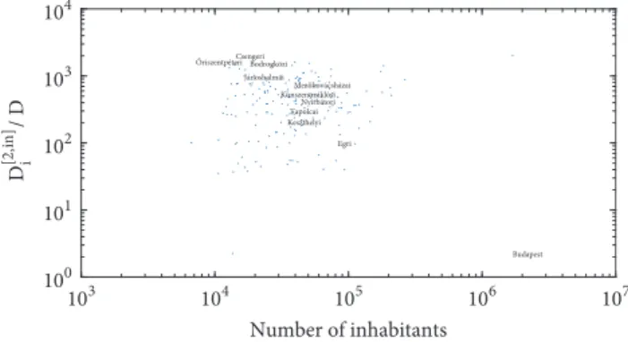
Figure 3: Network density as a function of the number of inhabi- tants on the level LAU 1.
company-ownership network. As shown in Figure 3, these densities are significantly higher in most subregions and a negative correlation exists between the size of the regions and the number of their inner connections (𝑟 = 0.298, 𝑝 < 10−4). As illustrated by the results, smaller locations are much more isolated than larger ones, like Budapest.
The same result is obtained by the analysis of the external density-based opennes measure which we consider as a main measure of attractiveness (see Appendix A for more details).
As shown in Figure 4, bigger regions exhibit lager openness values reflecting their higher degree of attractiveness (𝑟 = 0.94,𝑝 < 10−10).
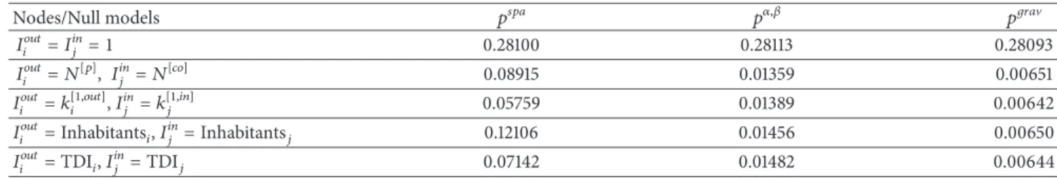
Table 2: Performances of distance-dependent null models.
Nodes/Null models 𝑝𝑠𝑝𝑎 𝑝𝛼,𝛽 𝑝𝑔𝑟𝑎V
𝐼𝑖𝑜𝑢𝑡= 𝐼𝑗𝑖𝑛= 1 0.28100 0.28113 0.28093
𝐼𝑖𝑜𝑢𝑡= 𝑁[𝑝], 𝐼𝑗𝑖𝑛= 𝑁[𝑐𝑜] 0.08915 0.01359 0.00651
𝐼𝑖𝑜𝑢𝑡= 𝑘[1,𝑜𝑢𝑡]𝑖 ,𝐼𝑗𝑖𝑛= 𝑘[1,𝑖𝑛]𝑗 0.05759 0.01389 0.00642
𝐼𝑖𝑜𝑢𝑡=Inhabitants𝑖,𝐼𝑗𝑖𝑛=Inhabitants𝑗 0.12106 0.01456 0.00650
𝐼𝑖𝑜𝑢𝑡=TDI𝑖,𝐼𝑗𝑖𝑛=TDI𝑗 0.07142 0.01482 0.00644
Budapest
Nagykátai
Ózdi Siklósi
Karcagi Devecseri
Bácsalmási
Vasvári
Budaörsi Ráckevei
Kiskőrösi
104
103 105 106 107
Number of inhabitants 10−4
10−3 10−2 10−1 100
$[2,?R] C/$[2,CH] C
Figure 4: Openness of small regions (LAU 1 level) as a function of the number of their inhabitants.
without Budapest connections with Budapest Total
104 105 106 107 108 109
Deterrence function, f(>C,D)
50 100 150 200 250 300 350
0
Distance [km]
Figure 5: Empirically derived deterrence function determined by (19), where𝐼𝑖[𝑖𝑛]= 𝑛[1,𝑝]𝑖 , 𝐼𝑗[𝑖𝑛]= 𝑛[1,𝑐𝑜]𝑗 .
3.3. The Effect of Geographical Distance. To address the effect of distance decay on link formation, the observed ties between the towns were compared with their expected number calculated from a probabilistic model.
A resolution of 10 km was used for binning the distance distribution (see Figure 5). The exponent of distance decay according to our data is -1.1057. It should be noted that the effect of the capital city is so high, the probability of forming connections with Budapest is slightly less distance- dependent, and the exponent of distance decay with regard to these connections is only -0.6385.
The distance-dependent link formation probability can be explained by the notion that the costs of establishing and
maintaining the connections are also distance-dependent.
This assumption can be confirmed by the fact that the distance has a much stronger effect on investment ties than on online social networks in Hungary (where the exponent of distance decay is -0.6) [44], probably since the cost of keeping connections is less dependent on distance than the management of a company far from the permanent address of the owner.
3.4. Comparison of the Null Models. Based on the utilized distance function, three different types of models can be defined. When𝑓(𝑑)is a deterrence function defined by (19), the models are denoted as 𝑝𝑠𝑝𝑎 = 𝛾𝐼𝑖𝑜𝑢𝑡𝐼𝑖𝑛𝑗𝑓(𝑑). 𝑝𝛼,𝛽 = 𝛾(𝐼𝑖𝑜𝑢𝑡)𝛼(𝐼𝑗𝑖𝑛)𝛽𝑓(𝑑)represents the parametric version of this model, when the exponents𝛼and𝛽are optimized to achieve a more accurate approximation of connections between towns.𝑝𝑔𝑟𝑎V𝑖,𝑗 = 𝛾(𝐼𝑖𝑜𝑢𝑡)𝛼(𝐼𝑗𝑖𝑛)𝛽/𝑑𝛿represents the gravity-type models.
Five sets of 𝐼𝑖𝑜𝑢𝑡, 𝐼𝑗𝑖𝑛 variables were defined, including simple metrics like the numbers of nodes and edges [1]
in addition to socioeconomic variables, like the number of inhabitants and Total Domestic Income (total income received by all sectors of the economy including the sum of all wages, profits, and taxes, minus subsidies). Based on the combination of different variables and distance functions, 15 different models were identified:
min𝛼,𝛽,𝛾𝐸𝑚(𝛼, 𝛽, 𝛾) = 1
𝐿A[1]−P[1]2. (23) As summarized in Table 2, by taking the distance into account, the accuracy of the model is significantly improved.
Among distance-dependent models, the gravity models per- form best (in comparison, the accuracy of the distance independent random configuration model is 0.16494).
The Total Domestic Income (TDI) is one of the best indicators. The identified 𝛼, 𝛽, and𝛿parameters reflect the importance of the𝐼𝑜𝑢𝑡𝑖 , 𝐼𝑗𝑖𝑛, and𝑑variables in the models (e.g., in the case where𝐼𝑗𝑖𝑛 = 𝑇𝐷𝐼𝑗and𝐼𝑖𝑜𝑢𝑡 = 𝑇𝐷𝐼𝑖, the resultant nonlinear regression model is 𝑝𝑖,𝑗 = 0.12 ⋅ ((𝐼𝑖𝑜𝑢𝑡)0.37 ⋅ (𝐼𝑗𝑖𝑛)0.81)/𝑑1.58(see Table 3)), which can be interpreted as the notion that the number of connections between location𝑖and location𝑗is increased by0.37% as a result of1.0% growth of TDI in location 𝑖. Similarly, the number of connections between location𝑖and location𝑗is increased by0.81% as a result of1.0% growth of TDI in location𝑗. According to the gravity-type models, the importance of the target/destination
Table 3: Coefficients of the parametric models that reflect the importance of the variables.
𝑝𝛼,𝛽= 𝛾 (𝐼𝑖𝑜𝑢𝑡)𝛼(𝐼𝑗𝑖𝑛)𝛽𝑓(𝑑) 𝑝𝑖,𝑗𝑔𝑟𝑎V= 𝛾 (𝐼𝑖𝑜𝑢𝑡)𝛼(𝐼𝑗𝑖𝑛)𝛽/𝑑𝛿
Nodes/Parameters 𝛼 𝛽 𝛼 𝛽 𝛿
𝐼𝑖𝑜𝑢𝑡= 𝑁[𝑝],𝐼𝑗𝑖𝑛= 𝑁[𝑐𝑜] 1.08373 0.91787 0.34984 0.67191 1.63711
𝐼𝑖𝑜𝑢𝑡= 𝑘[1,𝑜𝑢𝑡]𝑖 ,𝐼𝑗𝑖𝑛= 𝑘[1,𝑖𝑛]𝑗 1.05439 0.94455 0.35652 0.69045 1.59439
𝐼𝑖𝑜𝑢𝑡=Inhabitants𝑖,𝐼𝑗𝑖𝑛=Inhabitants𝑗 0.99347 1.15642 0.40654 0.88313 1.52391
𝐼i𝑜𝑢𝑡= 𝑇𝐷𝐼𝑖,𝐼𝑗𝑖𝑛= 𝑇𝐷𝐼𝑗 0.98571 1.03669 0.37367 0.81425 1.58060
105
100
105
100
105
100
105
100
0.' C,D
0, C,D 03J; C,D0'L;P C,D
A
106 104
102 100
A
106 104
102 100
A
106 104
102 100
A
106 104
102 100
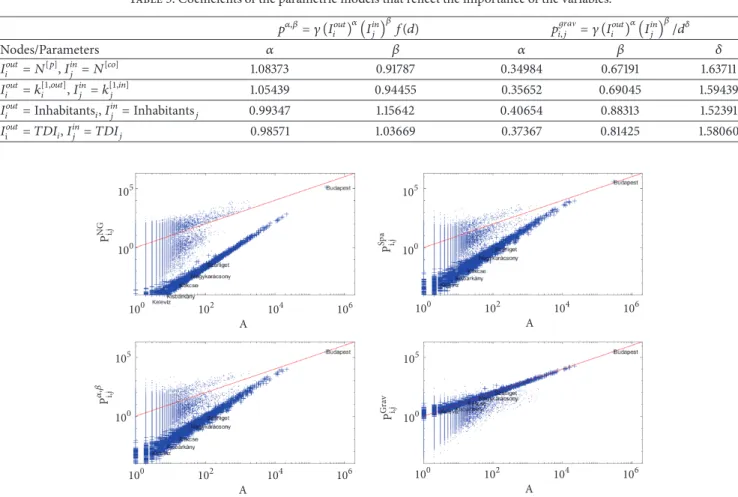
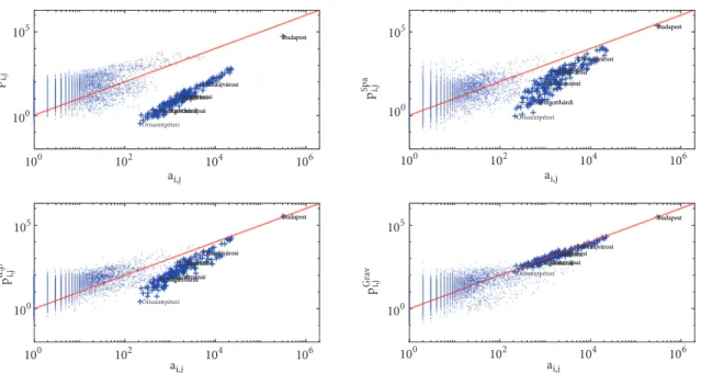
Figure 6: Comparison between the number of the edge weights𝑎𝑖,𝑗[1]and their estimated values𝑝[1]𝑖,𝑗 generated by different null models on the town level (LAU 2) settlement hierarchy when𝐼𝑖𝑜𝑢𝑡= 𝑘[1,𝑜𝑢𝑡]𝑖 and𝐼𝑗𝑖𝑛= 𝑘[1,𝑖𝑛]𝑗 . The + symbols represent the inner connections that form a separate cluster. This plot directly reflects the goodness of fit as the model estimates the connections of the towns.
locations (𝛽) is greater than the importance of the sources (𝛼) regardless of how the strengths of the nodes are interpreted.
3.5. Evaluation of the Modularities. As modularity-based community detection evaluates the set of𝑎𝑖,𝑗[1] > 𝑝𝑖,𝑗[1]edges (and the related nodes) whose weights are underestimated by the null model (see (11)), we designed a plot that compares 𝑎𝑖,𝑗[1]with𝑝𝑖,𝑗[1]to highlight the set of potential edges that can be used to form communities.
Four null models based on the𝐼1fl𝑘[1,𝑜𝑢𝑡]𝑖 and𝐼2fl𝑘[1,𝑖𝑛]𝑗 Newman and Girvan model are compared in Figure 6. In all models, the inner connections (represented by +) form a separate cluster which confirms that74% of the connections remain within the borders of the towns. The first model (𝑝𝑁𝐺) shows that more inner connections exist than would be expected based on the random configuration network.
The spatial models𝑝𝑆𝑝𝑎𝑡and𝑝𝛼,𝛽handle the dependence on distance of the connections, so a slightly smaller difference is shown in the number of the experienced and expected inner connections. It is reflected in Figure 7 that during the aggregation procedure the qualitative behavior of the models does not change.
The difference between the expected number of intercon- nections is higher in the case of smaller settlements which indicates that small regions are not as attractive as would be expected from their number of nodes. The gravity model 𝑝𝐺𝑟𝑎V well estimates the inner connections thanks to the exponents𝛼 = 0.35652and𝛽 = 0.69045whose parameters effectively represent that the increase in the number of connections affects the attractiveness in a nonlinear fashion.
This phenomenon is much more interesting when the utilized variables can be interpreted as economic potentials. When TDI is applied in the gravity model, 𝛼 = 0.37367 and 𝛽 = 0.81425. These values and Figure 8 confirm that gravity- based models behave similarly and, therefore, reflect the same mechanism of attractiveness.
3.6. Forming Communities. Connections that interlink com- munities are indicative of their relationships. The effect of these interlinks can be studied by the change in modularity (see (21)) expressed asΔM[𝑙] = (B[𝑙])𝑇+B[𝑙].
To determine the community structure, the MATLAB implementation [49] of the greedy Louvain algorithm [50]
was used. Towns and subregions were used as an initial
Budapest
Dunaújvárosi Szentesi Tiszaújvárosi Kiskunmajsai Szentgotthárdi
Budapest
Dunaújvárosi Szentesi Tiszaújvárosi Kiskunmajsai Szentgotthárdi
Budapest
Dunaújvárosi Szentesi Tiszaújvárosi Kiskunmajsai
Szentgotthárdi
Budapest
Dunaújvárosi Szentesi Tiszaújvárosi Kiskunmajsai
Szentgotthárdi
Budapest
Dunaújvárosi Szentesi Tiszaújvárosi Kiskunmajsai Szentgotthárdi
Dunaújvárosi Szentesi Tiszaújvárosi Kiskunmajsai Szentgotthárdi
Budapest
Dunaújvárosi Szentesi Tiszaújvárosi Kiskunmajsai Szentgotthárdi
Budapest
Dunaújvárosi Szentesi Tiszaújvárosi Kiskunmajsai Szentgotthárdi Budapest
105
100
105
100
105
100
105
100
p.' C,D
p, C,D p3J; C,Dp'L;P C,D
106 104
102 100
106 104
102 100
106 104
102 100
106 104
102
100 ;C,D
;C,D
;C,D
;C,D
Őriszentpéteri
Őriszentpéteri
Őriszentpéteri Őriszentpéteri
Figure 7: Comparison between the number of the edge weights𝑎𝑖,𝑗[2]and their estimated values𝑝𝑖,𝑗[2]generated by different null models at level LAU 1 of the settlement hierarchy when𝐼𝑖𝑜𝑢𝑡 = 𝑘[1,𝑜𝑢𝑡]𝑖 and𝐼𝑗𝑖𝑛 = 𝑘[1,𝑖𝑛]𝑗 . The + symbols represent the inner connections that form a separate cluster. This plot reflects that, during the aggregation procedure, the qualitative behavior of the models does not change; furthermore, the same phenomena can be observed as in Figure 6.
Budapest
Dunaújvárosi Szentesi Tiszaújvárosi Kiskunmajsai Szentgotthárdi
Budapest
Dunaújvárosi Szentesi Tiszaújvárosi Kiskunmajsai Szentgotthárdi
10−2 10−1 100 101 102 103 104 105 106
p'L;P C,D
101 102 103 105 106
100 104
;C,D
Őriszentpéteri
Figure 8: Comparison between the number of the edge weights𝑎[2]𝑖,𝑗 and their estimated values𝑝𝑖,𝑗[2]generated by the gravity null model at level LAU 1 of the settlement hierarchy when𝐼𝑖𝑜𝑢𝑡 = 𝑇𝐷𝐼𝑖and 𝐼𝑗𝑖𝑛= 𝑇𝐷𝐼𝑗. The + symbols represent the inner connections that form a separate cluster.
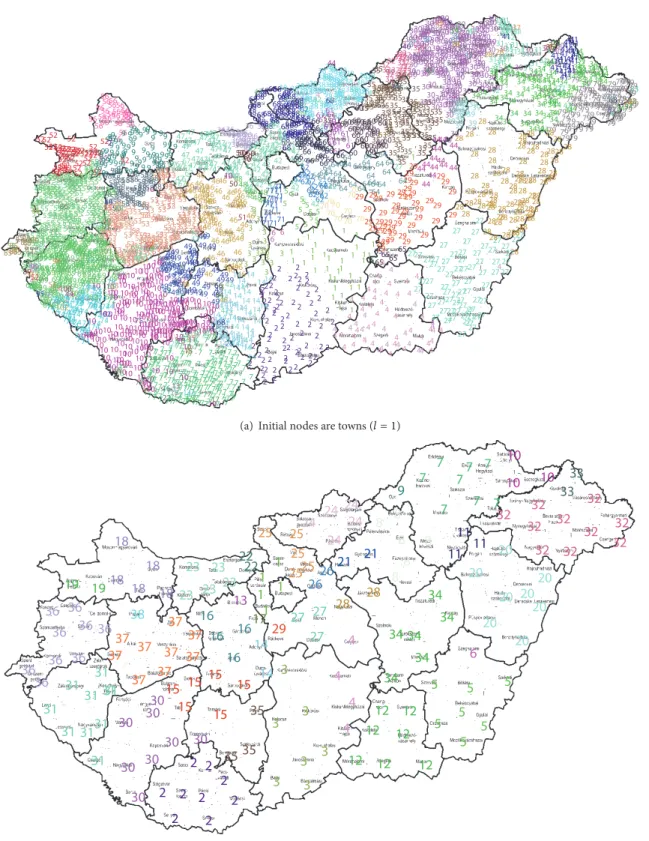
partition B[𝑙]. As shown in Figure 9, the community struc- ture formed based on the null model 𝑝𝑁𝐺 almost per- fectly reconstructs the counties confirming that the settle- ment structure is reflected in terms of the personal invest- ments.
Different null models provide different viewpoints with regard to community detection. The NG null model does not handle the distance dependence of the connections so the matrix B[𝑙] = A[𝑙] − P[𝑙] of the modeling errors reflects the distance dependence of the connections. There- fore, the resulting communities form spatial clusters. On the contrary, communities formed by the gravitational models
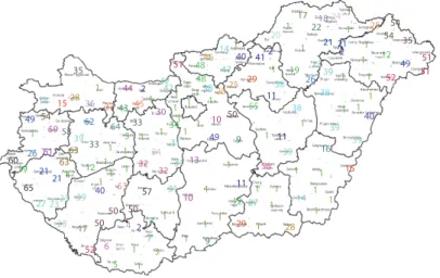
reflect distance-dependent differences less. According to the resultant maps, the attractiveness of Budapest is highlighted as only small since closed regions were not assigned to the module of the capital (see Figure 10(a)). It is interesting to note that all the centers of counties were assigned to the community of Budapest in gravitational model which also confirms the hierarchical structure of the network. To high- light the hierarchical structure and increase the sensitivity of the model, a resolution parameter was introduced into the model (see Appendix B) that can be adapted to detect similar region-pairs as shown in Figure 10(b).
Communities formed with the NG null model (see Figure 9) and the TDI-based gravity models (see Figure 10) significantly differ. The interpretation of the communities and these differences should rely on the understanding of the concept of the modularity. The utilised modularity detection algorithm generates partitions in which the links are more abundant within communities than would be expected from the employed model.
As the NG null model only uses the basic structural information encoded in the adjacency matrix, when the probabilities of the connections are dependent on distance, the resulting communities will represent closer geographical regions. As Table 1 and Figures 6 and 7 show, most of the connections remain within the county borders, so it is natural that the resultant 30 communities are almost identical to the counties.
Since the Hungarian road network reflects the admin- istrative regions, it can be shown that the distance strongly affects the probability of the connections. This distance dependence of the connection probability can be incorpo- rated into the null model by the proposed gravity model.
(a) Initial nodes are towns (𝑙 = 1)
(b) Initial nodes are subregions (𝑙 = 2)
Figure 9: Communities formed by the Louvain method and Newman-Girvan (NG) null model (𝐼𝑖= 𝑘𝑜𝑢𝑡𝑖 and𝐼𝑗= 𝑘𝑖𝑛𝑗) reflect the settlement hierarchy as the resultant communities are almost identical to the counties.
In this case, the resultant communities will reflect another unmodelled surplus in the number of connections. When the attractiveness and the distances are considered in the null model, the communities will reflect the additional economic attractiveness/similarity of the regions.
As Figure 10 shows, the algorithm generates a huge cluster of a well developed regions with Budapest, the larger cities and county seats with high TDIs, and several small communities related to isolated and less developed subre- gions.
(a) TDI-based gravitational model: Initial nodes are subregions (𝑙 = 2)
(b) The same TDI-based gravitational model at higher resolution𝛾𝑟= 1.1
42 520
520 646
646 771
771 897
897 1266
−
−
−
−
−
(c) Spatial distribution of the TDI per capita (in 1000 HUF)
Figure 10: Communities formed by the Louvain method and gravitational null models reflect the attractiveness of Budapest as only less developed closed regions were not assigned to the module of the capital.
4. Conclusions
Regional policy-making and monitoring are firm-centered, incentive-based, and state-driven. Personal investments define ties between geographical locations. We analyzed the structure of this ownership network and proposed a methodology to characterize regional attractiveness based on a set of null models identified to approximate the probabilities of link formation. According to the levels of the settlement hierarchy, a four-level study was conduct- ed.
Based on the calculation of the internal and exter- nal network densities, several measures were proposed to evaluate the attractiveness and development of towns and geographical regions. The results indicate that small and less competitive regions have less internal connections, while larger cities are much more open.
To provide a more in-depth insight into the network, the dependence of link formation on distance was studied.
The probability of connections between owners and their companies shows a much more rapid degree of distance decay than experienced in social networks. The attractiveness of the capital is so high that its connections are much less dependent on distance than other cities.
Based on the combination of three deterrence models and five sets of indicators, 15 different null models were identified besides the classical Newman-Girvan random configuration model. Communities statistically have more significant edge weights that would be wired according to the null model. As it was highlighted that underestimated link probabilities are the sources of modularity, a scatter plot was designed to visualize how the null model approximates the real structure of the network.
The identification of gravity-type models highlighted that link formation is nonlinearly dependent on the studied variables. Furthermore, the target nodes are much more important when determining the probability of link forma- tion than the source nodes which also confirms why the structural analysis of company-ownership networks can be used to measure regional attractiveness.
We applied the Louvain community detection algorithm to form clusters of cities and subregions and compared the resultant communities to administrative regions. When the null model more closely approximates the real structure of the network, then the modularity is expected to be lower.
As community detection forms modules whose internal link densities are significantly higher than what would be expected from the applied null models, spatial clusters that were highlighted by the distance independent random configuration model are almost identical to the counties.
Communities generated based on the gravitational models, which correctly estimate the number of internal nodes and the dependence of link formation on distance, exploited the attractiveness of the capital, as they form a massive cluster that includes most of the centers of each county, bigger cities, and the competitive touristic regions, while the remaining small clusters reflect isolated regions that are less developed and less attractive.
Appendix
A. Internal and External
Connection-Based Evaluation
Finding community structure means the assignment of the nodes into groups, where within the nodes are highly con- nected and across the nodes of the communities they are much loosely connected to each other [51].
The density of the whole network can be calculated as
𝐷 = 𝐿
𝑁[𝑝]𝑁[𝑐𝑜]. (A.1)
while the internal density of the region is calculated as 𝐷[𝑙,𝑖𝑛]𝑖 = 𝑎𝑖,𝑖[𝑙]
𝑛[𝑙,𝑝]𝑖 𝑛[𝑙,𝑐𝑜]𝑖 . (A.2)
𝐷[𝑙,𝑖𝑛]𝑖 /𝐷compares internal complexity of the regions to the whole network.
The probability of an external tie, in other words, the external density, can be calculated in a similar fashion:
𝐷[𝑙,𝑒𝑥]𝑖 = ∑𝑖 ̸=𝑗𝑎𝑖,𝑗[𝑙]
𝑁[𝑙,𝑝](𝑁[𝑙,𝑐𝑜]− 𝑛[𝑙,𝑐𝑜]𝑖 ), (A.3) where 𝑁[𝑙,𝑐𝑜] − 𝑛[𝑙,𝑐𝑜]𝑖 represents the number of companies that are outside of the𝑖-th region at the [𝑙]-th level of the settlement hierarchy.
To evaluate the openness as a measure of the attrac- tiveness of the region, the ratio of the external to internal probabilities can be defined as
𝑂[𝑙]𝑖 = 𝐷[𝑙,e𝑥]𝑖
𝐷[𝑙,𝑖𝑛]𝑖 . (A.4)
Apart from taking into account internal and external links, the direction of the connections can be considered.
Expansion computes the number of edges pointing outside the community [37]:
𝐸[𝑙]𝑖 = ∑𝑖𝑎[𝑙]𝑖,𝑗− ∑𝑖𝑎𝑖,𝑖[𝑙]
𝑛[𝑙,𝑝]𝑖 . (A.5)
Similarly, the ability of a community to collects links can be determined by the normalized number of links that point inside the community:
𝐿𝐶𝐴[𝑙]𝑖 = ∑𝑗𝑎[𝑙]𝑖,𝑗− 𝑎[𝑙]𝑖,𝑖
𝑛[𝑙,𝑐𝑜]𝑖 . (A.6)
Cut ratio is similar to the internal density as it computes the fraction of edges pointing out and the number of possible edges that are pointing outside the community:
𝐶𝑅[𝑙]𝑖 = ∑𝑗𝑎𝑖,𝑗[𝑙]− 𝑎𝑖,𝑖[𝑙]
𝑛[𝑙,𝑝]𝑖 (𝑁[𝑙,𝑐𝑜]− 𝑛[𝑙,𝑐𝑜]𝑖 ). (A.7)