arXiv:1512.06848v3 [math.AG] 1 Feb 2018
EULER CHARACTERISTICS OF HILBERT SCHEMES OF POINTS ON SIMPLE SURFACE SINGULARITIES
AD ´´ AM GYENGE, ANDR ´AS N´EMETHI, AND BAL ´AZS SZENDR ˝OI
Abstract. We study the geometry and topology of Hilbert schemes of points on the orbifold surface [C2/G], respectively the singular quotient surfaceC2/G, whereG <SL(2,C) is a finite subgroup of typeAorD. We give a decomposition of the (equivariant) Hilbert scheme of the orbifold into affine space strata indexed by a certain combinatorial set, the set of Young walls.
The generating series of Euler characteristics of Hilbert schemes of points of the singular surface of typeAorDis computed in terms of an explicit formula involving a specialized character of the basic representation of the corresponding affine Lie algebra; we conjecture that the same result holds also in type E. Our results are consistent with known results in typeA, and are new for typeD.
Contents
1. Orbifold singularities and their Hilbert schemes 2
1.1. Quotient surface singularities, Hilbert schemes and generating series 2
1.2. Simple surface singularities 3
1.3. Some terminology and structure of the paper 5
Acknowledgements 5
2. Type An 5
2.1. TypeAbasics 5
2.2. Partitions, torus-fixed points and decompositions 5
2.3. Abacus of typeAn 7
2.4. Relating partitions to 0-generated partitions 8
3. Type Dn: ideals and Young walls 10
3.1. The binary dihedral group 10
3.2. Young wall pattern and Young walls 11
3.3. Decomposition ofC[x, y] and the transformed Young wall pattern 12
3.4. Subspaces and operators 12
3.5. Cell decompositions of equivariant Grassmannians 13
3.6. The Young wall associated to a homogeneous ideal 15
4. Type Dn: decomposition of the orbifold Hilbert scheme 16
4.1. The decomposition 16
4.2. Incidence varieties 19
4.3. Proof of Theorem 4.3 21
4.4. Preparation for the proof of the incidence propositions 24
4.5. Proofs of propositions about incidence vareties 29
5. Type Dn: special loci 31
5.1. Support blocks 31
5.2. Special loci in orbifold strata and the supporting rules 32
5.3. Special loci in Grassmannians 33
5.4. Proof of Theorem 5.2 35
6. Type Dn: decomposition of the coarse Hilbert scheme 36
6.1. Distinguished 0-generated Young walls 36
6.2. The decomposition of the coarse Hilbert scheme 39
6.3. Possibly and almost invariant ideals 40
6.4. Euler characteristics of strata and the coarse generating series 42
1991 Mathematics Subject Classification. Primary 14N10; Secondary 05E10.
Key words and phrases. Hilbert scheme, singularities, Euler characteristic, generating series, Young wall.
1
7. Type Dn: abacus combinatorics 46
7.1. Young walls and abacus of type Dn 46
7.2. Core Young walls and their abacus representation 47
7.3. 0-generated Young walls and their abacus representations 49 7.4. The generating series of distinguished 0-generated walls 50
Appendix A. Background on representation theory 54
A.1. Affine Lie algebras and extended basic representations 54
A.2. Affine crystals 55
A.3. Affine Lie algebras and Hilbert schemes 55
Appendix B. Joins 55
References 56
1. Orbifold singularities and their Hilbert schemes
1.1. Quotient surface singularities, Hilbert schemes and generating series. Let G <
GL(2,C) be a finite subgroup and denote by C2/G the corresponding quotient variety. There are two different types of Hilbert scheme attached to this data. First, there is the classical Hilbert scheme Hilb(C2/G) of the quotient space. This is the moduli space of ideals in OC2/G(C2/G) = C[x, y]G of finite colength. We call this thecoarse Hilbert scheme of points. It decomposes as
Hilb(C2/G) = G
m∈N
Hilbm(C2/G)
into components that are quasiprojective but singular varieties indexed by “the number of points”, the codimensionmof the ideal. Second, there is the moduli space of G-invariant finite colength subschemes ofC2, the invariant part of Hilb(C2) under the lifted action ofG. This Hilbert scheme is also well known and is variously called the orbifold Hilbert scheme [43] orequivariant Hilbert scheme [18]. We denote it by Hilb([C2/G]). This space also decomposes as
Hilb([C2/G]) = G
ρ∈Rep(G)
Hilbρ([C2/G]), where
Hilbρ([C2/G]) ={I∈Hilb(C2)G: H0(OC2/I)≃Gρ}
for any finite-dimensional representationρ∈Rep(G) ofG; here Hilb(C2)Gis the set ofG-invariant ideals ofC[x, y], and≃GmeansG-equivariant isomorphism. Being components of fixed point sets of a finite group acting on smooth quasiprojective varieties, the orbifold Hilbert schemes themselves are smooth and quasiprojective [5].
There is a natural pushforward map between the two kinds of Hilbert scheme: each J ∈ Hilb([C2/G]) can be mapped to its G-invariant part, giving a morphism [4, 3.4]
p∗: Hilb([C2/G]) → Hilb(C2/G) J 7→ JG=J ∩C[x, y]G
called thequotient-scheme map. There is also a set-theoretic pullback map, which however does notpreserve flatness in families, so it is not a morphism between the Hilbert schemes: the inclusion i:C[x, y]G⊂C[x, y] induces a pullback map on the ideals, and its image is contained in the set of G-equivariant ideals, leading to a map of sets
i∗: Hilb(C2/G)(C) → Hilb([C2/G])(C) I 7→ i∗I=C[x, y].I
Since forIC[x, y]G, we clearly have (C[x, y].I)G =I, the compositep∗◦i∗is the identity on the set of ideals of the invariant ring.
We collect the topological Euler characteristics of the two versions of the Hilbert scheme into two generating functions. Letρ0, . . . , ρn∈Rep(G) denote the (isomorphism classes of) irreducible representations ofG, withρ0 the trivial representation.
Definition 1.1. (a) Theorbifold generating series of the orbifold [C2/G] is Z[C2/G](q0, . . . , qn) =
X∞ m0,...,mn=0
χ Hilbm0ρ0+...+mnρn([C2/G])
q0m0·. . .·qmnn.
(b) Thecoarse generating series of the singularityC2/Gis ZC2/G(q) =
X∞ m=0
χ Hilbm(C2/G) qm.
Remark 1.2. For a smooth varietyX, the generating series ZX(q) =
X∞ m=0
χ(Hilbm(X))qm
of the Euler characteristics of Hilbert schemes of points of X, as well as various refinements of this series, have been extensively studied. In particular, for a nonsingular curve C, we have MacDonald’s result [32]
ZC(q) = (1−q)−χ(C),
whereas for a nonsingular surfaceS we have (a specialization of) G¨ottsche’s formula [16]
(1) ZS(q) =
Y∞ m=1
(1−qm)−1
!χ(S)
. There are also results for higher-dimensional varieties [6].
For singular varieties X, the seriesZX(q) is much less studied. For a singular curveC with a finite set{P1, . . . , Pk}of planar singularities however, we have the beautiful conjecture of Oblomkov and Shende [39], proved by Maulik [33], which takes the form
(2) ZC(q) = (1−q)−χ(C)
Yk j=1
Z(Pi,C)(q).
Here Z(Pi,C)(q) are highly nontrivial local terms that depend only on the embedded topological type of the link of the singularityPi∈C.
1.2. Simple surface singularities. In this paper we are only concerned with finite subgroups G <SL(2,C). See [19] for some partial results for some other finite groups. As it is well known, finite subgroups of SL(2,C) are classified into three types: typeAn for n≥1, typeDn forn≥4 and type En for n = 6,7,8. The type of the singularity can be parametrized by a simply-laced irreducible Dynkin diagram withnnodes, arising from an irreducible simply laced root system ∆.
We denote the corresponding group byG∆<SL(2,C); all other data corresponding to the chosen type will also be labelled by the subscript ∆. Irreducible representations ρ0, . . . , ρn of G∆ are then labelled by vertices of the affine Dynkin diagram associated with ∆. The singularityC2/G∆
is known as a simple (Kleinian, surface) singularity; we will refer to the corresponding orbifold [C2/G∆] as the simple singularity orbifold.
As we recall in Appendix A.3, the following result is known.
Theorem 1.3 ([37]). Let [C2/G∆] be a simple singularity orbifold. Then its orbifold generating series can be expressed as
(3) Z[C2/G∆](q0, . . . , qn) = Y∞ m=1
(1−qm)−1
!n+1
· X
m=(m1,...,mn)∈Zn
q1m1· · · · ·qmnn(q1/2)m⊤·C∆·m, whereq=Qn
i=0qidi withdi= dimρi, andC∆ is the finite type Cartan matrix corresponding to∆.
Our first main result is a strengthening of this theorem. Given a Dynkin diagram ∆ of typeA orD, we will recall below in 2.2, respectively 3.2, the definition of a certain combinatorial set, the set of Young wallsZ∆ of type ∆.
Theorem 1.4. Let[C2/G∆] be a simple singularity orbifold, where∆ is of type An for n≥1 or Dn for n≥4. Then there exists a decomposition
Hilb([C2/G∆]) = G
Y∈Z∆
Hilb([C2/G∆])Y
into locally closed strata indexed by the set of Young wallsZ∆of the appropriate type. Each stratum is isomorphic to an affine space of a certain dimension, and in particular has Euler characteristic χ(Hilb([C2/G∆])Y) = 1.
For type A, the set of Young walls is simply the set of finite partitions, represented as Young diagrams, equipped with a diagonal labelling. In this case, Theorem 1.4 is well known; the decom- position in type A is not unique, but depends on a choice of a one-dimensional subtorus of the full torus (C∗)2 acting on the affine planeC2. For completeness, we summarize the details in 2.2.
On the other hand, the typeD case appears to be new; in this case, our decomposition is unique, there is no further choice to make.
Remark 1.5. The orbifold Hilbert schemes of points for G < SL(2,C) are well known to be Nakajima quiver varieties for the corresponding affine quiver. As it was shown in [40], certain Lagrangian subvarieties in Nakajima quiver varieties are isomorphic to quiver Grassmannians for the preprojective algebra of the same type, parametrizing submodules of certain fixed modules.
On the other hand, results of the recent papers [30, 31] imply that every quiver Grassmannian of a representation of a quiver of affine typeD has a decomposition into affine spaces. The relation between this decomposition and ours deserves further investigation.
As we will explain combinatorially in 2.3, respectively 7.2, and via representation theory in A.1- A.2, the right hand side of (3) enumerates the set of Young wallsZ∆of the appropriate type. Thus Theorem 1.4 implies Theorem 1.3.
Remark 1.6. In type A, it is easy to refine formula (3) to a formula involving the Betti num- bers [13], or the motives [18], of the orbifold Hilbert schemes. We leave the study of such a refinement in typeD to future work; compare Remark 4.4.
The second main result of our paper is the following formula, which says that the coarse gener- ating series is a very particular specialization of the orbifold one.
Theorem 1.7. Let C2/G∆ be a simple singularity, where ∆ is of type An for n ≥1 or Dn for n≥4. Leth∨ be the (dual) Coxeter number of the corresponding finite root system (one less than the dimension of the corresponding simple Lie algebra divided by n). Then
ZC2/G∆(q) = Y∞ m=1
(1−qm)−1
!n+1
· X
m=(m1,...,mn)∈Zn
ζm1+m2+···+mn(q1/2)m⊤·C∆·m, whereζ= exp
2πi 1+h∨
andC∆ is the finite type Cartan matrix corresponding to∆.
ThusZC2/G∆(q) is obtained fromZ[C2/G∆](q0, . . . , qn) by the substitutions q1=· · ·=qn= exp
2πi 1 +h∨
, q0=qexp
− 2πi 1 +h∨
X
i6=0
dimρi
.
In typeA, the formula in Theorem 1.7 is not new: it was proved directly (in a slight disguise) by Dijkgraaf and Sulkowski in [8] and also recently, using completely different methods, by Toda in [42]. Our main contribution is the general Lie-theoretic formulation, as well as a proof in typeD;
we also provide a direct combinatorial proof in typeA, which appears to be new.
One can check directly that the generating series in Theorem 1.7 has also integer coefficients for E6,E7 andE8 to a high power inq. This motivates the following.
Conjecture 1.8. Let C2/G∆ be a simple singularity of type En for n = 6,7,8. Let h∨ be the (dual) Coxeter number of the corresponding finite root system. Then, as for other types,
ZC2/G∆(q) = Y∞ m=1
(1−qm)−1
!n+1
· X
m=(m1,...,mn)∈Zn
ζm1+m2+···+mn(q1/2)m⊤·C∆·m,
whereζ= exp
2πi 1+h∨
andC∆ is the finite type Cartan matrix corresponding to∆.
The key tool in our proof of Theorem 1.7 for typesAandDis the combinatorics of Young walls, in particular their abacus representation. We are not aware of such explicit combinatorics in type E. We hope to return to this question in later work.
Remark 1.9. We are dealing here with Hilbert schemes, parametrizing rankr= 1 sheaves on the orbifold or singular surface. In the relationship between the instantons on algebraic surfaces and affine Lie algebras, level equals rank [17]. Indeed the (extended) basic represenatation underlying the Young wall combinatorics (see Appendix) has levell= 1. Thus the substitution above is by the root of unityζ= exp
2πi l+h∨
, withl= 1 andh∨the (dual) Coxeter number. There is an intriguing analogy here with the Verlinde formula, which uses a similar substitution, into characters of Lie algebras, by a root of unityζ = exp(l+h2πi∨), wherel again is the level, and h∨ the (dual) Coxeter number of the root system of the Lie algebra of the gauge group. The geometric significance of this observation, if any, is left for future research.
Remark 1.10. Given the results above, it is easy to write down a global formula analogous to (2) for a singular surface with canonical singularities. This formula, as well as its modularity, are discussed in the announcement [21].
1.3. Some terminology and structure of the paper. We work over the fieldC of complex numbers. We call a regular map f: X →Y a trivial affine fibration with fibreAk, if there is an isomorphismX ∼=Y ×Ak withf being the first projection.
The structure of the rest of the paper is as follows. In Section 2, we give a new proof of Theo- rem 1.7 in typeA, which has the advantage that it generelizes away from that case. The rest of the paper treats the case of typeD. In Section 3, we introduce Schubert-style cell decompositions of Grassmannians of homogeneous summands ofC[x, y]. In Section 4 we give a cell decomposition of the orbifold Hilbert scheme, proving Theorem 1.4. In Section 5, we discuss some special subsets of the strata and their geometry. A decomposition of the coarse Hilbert scheme is given in Sec- tion 6. In Section 7, the proof of Theorem 1.7 is completed using combinatorial enumeration. The representation theoretic background is briefly summarized in Appendix A. Some relevant facts on joins of projective varieties are discussed in Appendix B.
Acknowledgements. The authors would like to thank Gwyn Bellamy, Alastair Craw, Eugene Gorsky, Ian Grojnowski, Kevin McGerty, Iain Gordon, Tomas Nevins and Tam´as Szamuely for helpful comments and discussions. ´A.Gy. was partially supported by the Lend¨ulet program (Mo- mentum Programme) of the Hungarian Academy of Sciences and by ERC Advanced Grant LDT- Bud (awarded to Andr´as Stipsicz). A.N. was partially supported by OTKA Grants 100796 and K112735. B.Sz. was partially supported by EPSRC Programme Grant EP/I033343/1.
2. Type An
2.1. TypeAbasics. Let ∆ be the root system of typeAn. Choosing a primitive (n+ 1)-st root of unityω, the corresponding subgroupG∆ofSL(2,C), a cyclic subgroup of ordern+ 1, is generated by the matrix
σ=
ω 0 0 ω−1
.
All irreducible representations ofG∆are one dimensional, and they are simply given byρj:σ7→ωj, forj ∈ {0, . . . , n}. The corresponding McKay quiver is the cyclic Dynkin diagram of type Ae(1)n .
The group G∆ acts on C2; the quotient variety C2/G∆ has an An singularity at the origin.
The matrix σ clearly commutes with the diagonal two-torus T = (C∗)2, and so T acts on the quotient C2/G∆ and the orbifold [C2/G∆]. Consequently T also acts on the orbifold Hilbert scheme Hilb([C2/G∆]) and the (reduced) coarse Hilbert scheme Hilb(C2/G∆) as well.
2.2. Partitions, torus-fixed points and decompositions. Consider the setN×Nof pairs of non-negative integers; we will draw this set as a set of blocks on the plane, occupying the non- negative quadrant. Label blocks diagonally with (n+ 1) labels 0, . . . , nas in the picture; the block with coordinates (i, j) is labelled with (i−j) mod (n+ 1). We will call this thepattern of typeAn.
0 1 n−1 n
n 0 n−2n−1
0 1
n 0
1 2
0 1
... . ..
. . . . . .
...
LetP denote the set of partitions. Given a partition λ= (λ1, . . . , λk)∈ P, with λ1 ≥. . .≥λk
positive integers, we consider its Young (or Ferrers) diagram, the subset ofN×Nwhich consists of theλi lowest blocks in column i−1. The blocks inλalso get labelled by then+ 1 labels. Let Z∆ denote the resulting set of (n+ 1)-labelled partitions, including the empty partition. For a labelled partitionλ∈ Z∆, let wtj(λ) denote the number of blocks in λlabelledj, and define the multiweight ofλto be wt(λ) = (wt0(λ), . . . ,wtn(λ)).
Proposition 2.1. The torusT acts with isolated fixed points on Hilb([C2/G∆]), parametrized by the set Z∆ of (n+ 1)-labelled partitions. More precisely, for k0, . . . , kn non-negative integers and ρ=⊕nj=0ρ⊕ki i, theT-fixed points onHilbρ([C2/G∆])are parametrized by(n+ 1)-labelled partitions of multiweight (k0, . . . , kn).
Proof. We just sketch the proof, which is well known [10, 13]. It is clear that the T-fixed points on Hilb([C2/G∆]), which coincide with the T-fixed points on Hilb(C2), are the monomial ideals in C[x, y] of finite colength. The monomial ideals are enumerated in turn by Young diagrams of partitions. The labelling of each block gives the weight of the G∆-action on the corresponding
monomial, proving the refined statement.
Corollary 2.2. There exist a locally closed decomposition, depending on a choice specified below, of Hilb([C2/G∆]) into strata indexed by the set of (n+ 1)-labelled partitions. Each stratum is isomorphic to an affine space.
Proof. Again, this is well known [38]. Fixing a representation ρ, choose a sufficiently general one- dimensional subtorus T0 ⊂T which has positive weight on both x and y. For general T0 ⊂T, the fixed point set on Hilbρ([C2/G∆]) is unchanged and in particular consists of a finite number of isolated points. Choosing positive weights onx, y ensures that all limits of T0-orbits att = 0 in Hilb([C2/G∆]) exist, even though Hilbρ([C2/G∆]) is non-compact. Since Hilbρ([C2/G∆]) is smooth, the result follows by taking the Bia lynicki-Birula decomposition of Hilbρ([C2/G∆]) given
by theT0-action.
Denote by
Z∆(q0, . . . , qn) = X
λ∈Z∆
qwt(λ)
the generating series of (n+ 1)-labelled partitions, where we used multi-index notation qwt(λ)=
Yn i=0
qwti i(λ).
From either of the previous two statements, we immediately deduce the following.
Corollary 2.3. Let[C2/G∆]be a simple singularity orbifold of typeA. Then its orbifold generating series can be expressed as
(4) Z[C2/G∆](q0, . . . , qn) =Z∆(q0, . . . , qn).
According to [13] the generating series of (n+ 1)-labelled partitions has the following form:
(5) Z∆(q0, . . . , qn) = P∞
m=(m1,...,mn)∈Zkqm11· · · · ·qnmn(q1/2)m⊤·C·m Q∞
m=1(1−qm)n+1 ,
where q=q0· · · · ·qn andC is the (finite) Cartan matrix of type An; for a sketch proof, see the end of 2.3 below. In particular, (4) and (5) imply Theorem 1.3 for typeA.
We now turn to the coarse Hilbert scheme. Let us define a subset Z∆0 of the set of (n+ 1)- labelled partitionsZ∆ as follows. An (n+ 1)-labelled partitionλ∈ Z∆ will be called 0-generated (a slight misnomer, this should be really be “complement-0-generated”) if the complement of λ inside N×Ncan be completely covered by translates ofN×N to blocks labelled 0 contained in this complement. Equivalently, an (n+ 1)-labelled partition λ is 0-generated, if all its addable blocks (blocks whose addition gives another partition) are labelled 0. It is immediately seen that this condition is equivalent to the corresponding monomial idealIC[x, y] being generated by its invariant partI∩C[x, y]G∆. Indeed, we have the following.
Proposition 2.4. The torus T acts with isolated fixed points on Hilb(C2/G∆), which are in bijection with the set Z∆0 of 0-generated (n+ 1)-labelled partitions. More precisely, for a non- negative integerk, the T-fixed points on Hilbk(C2/G∆) are parametrized by 0-generated (n+ 1)- labelled partitionsλwith0-weight wt0(λ) =k.
Proof. This is immediate from the above discussion. The T-fixed points of Hilb(C2/G∆) are the monomial idealsIofC[x, y]G∆ of finite colength. InsideC[x, y], the ideals they generate correspond to partitions which are 0-generated. The ringC[x, y]G∆ has a basis consisting of monomials with corresponding blocks labelled 0 insideC[x, y]; thus the codimension of a monomial ideal I inside
C[x, y]G∆ is simply the number of blocks denoted 0.
Denoting by
Z∆0(q) = X
λ∈Z∆0
qwt0(λ)
the corresponding specialization of the generating series of 0-generated (n+ 1)-labelled partitions, we deduce the following.
Corollary 2.5. Let[C2/G∆]be a simple singularity orbifold of typeA. Then the coarse generating series can be expressed as
(6) ZC2/G∆(q) =Z∆0(q).
Proof of Theorem 1.7 for theAn case. The (dual) Coxeter number of the typeAn root system is h∨ = n+ 1. Thus Theorem 1.7 for this case follows from Corollary 2.5, formula (5), and the combinatorial Proposition 2.7 below, which computes the seriesZ∆0(q).
Remark 2.6. The single variable generating seriesZC2/G∆in typeAwas calculated by Toda in [42]
using threefold machinery including a flop formula for Donaldson–Thomas invariants of certain Calabi–Yau threefolds. He does not mention any connection to Lie theory. The combinatorics, and the one-variable formula forZ∆0(q), were already known to Dijkgraaf and Sulkowski [8]. They do not give the interpretation of the combinatorial formula in terms of Hilbert schemes, though they are clearly motivated by closely related ideas. Their proof is different, using the method of Andrews [2] in place of the abacus combinatorics we use below. We believe that already in type A, our new proof is preferable since it directly exhibits the clear connection between the orbifold and coarse generating series. Also, as we show later, this method generalizes away from typeA.
2.3. Abacus of type An. We now introduce some standard combinatorics related to the typeA root system, which will allow us to relate the generating seriesZ∆of (n+ 1)-labelled partitions to the specialized seriesZ∆0 of 0-generated partitions. We follow the notations of [29].
Theabacus of typeAn is the arrangement of the set of integers in (n+ 1) columns according to the following pattern.
... ... ... ...
−2n−1 −2n . . . −n−2 −n−1
−n −n+ 1 . . . −1 0
1 2 . . . n n+ 1
n+ 2 n+ 3 . . . 2n+ 1 2n+ 2
... ... ... ...
Each integer in this pattern is called aposition. For any integer 1≤k≤n+ 1 the set of positions in the k-th column of the abacus is called the k-th runner. An abacus configuration is a set of beads, denoted by, placed on the positions, with each position occupied by at most one bead.
To an (n+ 1)-labelled partition λ= (λ1, . . . , λk)∈ Z∆ we associate its abacus representation (sometimes also called Maya diagram) as follows: place a bead in position λi−i+ 1 for all i, interpretingλias 0 fori > k. Alternatively, the abacus representation can be described by tracing the outer profile of the Young diagram of a partition: the occupied positions occur where the profile moves “down”, whereas the empty positions are where the profile moves “right”. In the abacus representation of a partition, the number of occupied positive positions is always equal to the number of absent nonpositive positions; we call such abacus configurationsbalanced. Conversely, it is easy to see that any balanced configuration represents a unique (n+ 1)-labelled partition, an element ofZ∆.
Forn= 0, we obtain a representation of partitions on a single runner; this is sometimes called theDirac searepresentation of partitions.
The (n+ 1)-coreof a labelled partitionλ∈ Z∆is the partition obtained fromλby successively removing border strips of length n+ 1, leaving a partition at each step, until this is no longer possible. Here aborder stripis a skew Young diagram which does not contain 2×2 blocks and which contains exactly onej-labelled block for all labelsj. The removal of a border strip corresponds in the abacus representation to shifting one of the beads up on its runner, if there is an empty space on the runner above it. In this way, the core of a partition corresponds to the bead configuration in which all the beads are shifted up as much as possible; this in particular shows that the (n+ 1)-core of a partition is well-defined. We denote byC∆ the set of (n+ 1)-core partitions, and
c: Z∆→ C∆
the map which takes an (n+ 1)-labelled partition to its (n+ 1)-core.
Given an (n+ 1)-coreλ, we can read the (n+ 1) runners of its abacus rrepresentation separately.
These will not necessarily be balanced. Thei-th one will be shifted from the balanced position by a certain integer numberai steps, which is negative if the shift is toward the negative positions (upwards), and positive otherwise. These numbers satisfyPn
i=0ai = 0, since the original abacus configuration was balanced. The set{a1, . . . , an}completely determines the partition, so we get a bijection
(7) C∆←→
( n X
i=0
ai= 0 )
⊂Zn+1.
We will represent an (n+ 1)-core partition by the corresponding (n+ 1)-tuplea= (a0, . . . , an).
On the other hand, for an arbitrary partition, on each runner we have a partition up to shift, so we get a bijection
Z∆←→ C∆× Pn+1.
This corresponds to the structure of formula (5) above; its denominator is the generating series of (n+ 1)-tuples of (unlabelled) partitions, whereas its numerator (after eliminating a variable) is exactly a sum overa∈ C∆. The multiweight of a core partition corresponding to an elementais given by the quadratic expressionQ(a) in the exponent of the numerator of (5). For more details, see Bijections 1-2 in [14,§2].
2.4. Relating partitions to 0-generated partitions. The purpose of this section is to prove the following, completely combinatorial statement.
Proposition 2.7. Let∆be of typeAn, and letξbe a primitive(n+ 2)-nd root of unity. Then the generating series of0-generated partitions can be computed from that of all(n+ 1)-labelled ones by the following substitution:
Z∆0(q) =Z∆(q0, . . . , qn)
q0=ξ−nq,q1=···=qn=ξ.
We start by combinatorially relating partitions to 0-generated partitions. Z∆0 is clearly a subset ofZ∆, but there is also a map
p: Z∆→ Z∆0
defined as follows: for an arbitrary partition λ, let p(λ) be the smallest 0-generated partition containing it. Since the set of 0-generated partitions is closed under intersection, p(λ) is well- defined, and it can be constructed as follows:p(λ) is the complement of the unions of the translates of N×N to 0-labelled blocks in the complement of λ. It is clear that p(λ) can equivalently be obtained by adding all possible addable blocks toλof labels different from 0.
Remark 2.8. The map pcan also be described in the language of ideals. If the monomial ideal IC[x, y] corresponds to the partitionλ, then the monomial ideali∗p∗I= (I∩C[x, y]G∆).C[x, y]
C[x, y] corresponds to the partitionp(λ).
Lemma 2.9. The bead configurations corresponding to 0-generated partitions are exactly those which have all beads right-justified on each row, with no empty position to the right of a filled position. The mapp:Z∆ → Z∆0 can be described in the abacus representation by the process of pushing all beads of an abacus configuration as far right as possible.
Proof. This follows from the description of the map from a partition to its abacus representation using the profile of the partition. Indeed, a 0-generated partition has a profile which only turns from “down” to “right” at 0-labelled blocks. In other words, the only time when a string of filled positions can be followed by an empty position is when the last filled position is on the rightmost runner. In other words, there cannot be empty positions to the right of filled positions in a row.
The proof of the second statement is similar.
Remark 2.10. As explained above, the maps c: Z∆ → C∆ and p: Z∆ → Z∆0 have natural descriptions on abacus configurations: ccorresponds to pushing beads all the way up within their column, whereasp corresponds to pushing beads all the way to the right within their row. It is then clear that there is also a third map Z∆ →0Z∆ ⊂ Z∆, dual to p, defined on the abacus by pushing beads all the way to the left. On labelled partitions this corresponds to the operation of removing all possible blocks with labels different from 0. This dual constuction occured in the literature earlier in [15].
Proof of Proposition 2.7. We will prove the substitution formula on the fibres of the mapp:Z∆→ Z∆0. In other words, we need to show that for any givenλ0∈ Z∆0, we have
(8) X
µ∈p−1(λ0)
qwt(µ)
q1=···=qn=ξ,q0=ξ−nq =qwt0(λ0).
As a first step, we reduce the computation to 0-generated cores. Given an arbitrary 0-generated partition λ, by the first part of Lemma 2.9 its coreν = c(λ) is also 0-generated, and the corre- sponding abacus configuration can be obtained by permuting the rows of the configuration ofλ.
Fix one such permutationσof the rows. Then, using the second part of Lemma 2.9, we can use the row permutationσ to define a bijection
˜
σ:p−1(λ)→p−1(ν)
between (abacus representations of) partitions in the fibres, mappingλitself to ν.
The difference between the partitionsλandν is a certain number of border strips, each removal represented by pushing up one bead on some runner by one step. Each border strip contains one block of each label, so the total number of times we need to push up a bead by one step on the different runners isN = wt0(λ)−wt0(ν). Thus, withq=q0·. . .·qn as in the substitution above, we can write
qwt(λ)=qwt0(λ)−wt0(ν)qwt(ν).
On the other hand, it is easy to see that in fact for anyµ∈p−1(λ), the corresponding ˜σ(µ) can also be obtained by pushing up beads exactlyN times, one step at a time, the difference being just in the runners on which these shifts are performed. This means that eachµdiffers from ˜σ(µ) by the same numberN = wt(λ)−wt(ν) of border strips. Therefore, we have
X
µ∈p−1(λ)
qwt(µ)=qwt0(λ)−wt0(ν) X
µ∈p−1(ν)
qwt(µ).
This is clearly compatible with (8) and reduces the argument to 0-generated core partitions.
Fix a 0-generated coreλ∈ Z∆0∩C∆; using Lemma 2.9 again, the corresponding (n+ 1)-tuple is a set ofnondecreasingintegersa= (a0, . . . , an) summing to 0. The fibrep−1(λ) consists of partitions
whose abacus representation contains the same number of beads in each row asλ. The shift of one bead to the left results in the removal in the partition of a block labelledi, with 1≤i≤n. After substitution, this multiplies the contribution of the diagram on the right hand side of (8) byξ−1. If we fix all but one row, which containsk beads, then these contributions add up to
n−k+1X
n1=0 n1
X
n2=0
· · ·
nXk−1
nk=0
(ξ−1)n1+···+nk= n+ 1
k
ξ−1
, where mr
z=[r] [m]z!
z![m−r]z! is the Gaussian binomial coefficient, with [m]z= 1−z1−zm.
The number of rows containing exactly k beads in the configuration corresponding to λ is an+1−k−an−k. Therefore, the total contribution of the preimages, the left hand side of (8), is
X
µ∈p−1(λ)
qwt(µ)
q1=···=qn=ξ,q0=ξ−nq = Yn k=1
n+ 1 k
an+1−k−an−k
ξ−1
qwt(λ)
q1=···=qn=ξ,q0=ξ−nq
= Yn l=0
n+1 n+1−l
ξ−1 n+1 n−l
ξ−1
!al
qwt(λ)
q1=···=qn=ξ,q0=ξ−nq
= Yn l=0
1−ξ−l−1 1−ξl−n−1
al
qwt(λ)
q1=···=qn=ξ,q0=ξ−nq
= Yn l=1
1−ξ−n−1 1−ξ−1
1−ξ−l−1 1−ξl−n−1
al
qwt(λ)
q1=···=qn=ξ,q0=ξ−nq
=ξ−Pnl=1lalqwt(λ)
q1=···=qn=ξ,q0=ξ−nq, where in the second equality we used n+10
z = n+1n+1
z = 1, in the penultimate equality we used a0=−a1− · · · −an, and in the last equality we used
1−ξ−n−1 1−ξ−1
1−ξ−l−1
1−ξl−n−1 =ξ−l,
which can be checked to hold for ξ a primitive (n+ 2)-nd root of unity. Incidentally, as the multiplicative order ofξis exactlyn+ 2, all the denominators appearing above are non-vanishing.
Finally, according to [14,§2], we have
qwt(λ)=qQ(a)2 qa11+···+an·. . .·qann,
where again q = q0·. . .·qn and Q : Zn → Z is the quadratic form associated to C∆. Since q0
appears only inqon the right hand side, it is clear that Q(a)2 = wt0(λ). Hence, qQ(a)2 q1a1+···+an. . . qann
q1=···=qn=ξ =qwt0(λ)ξPnl=1lal.
This concludes the proof.
3. Type Dn: ideals and Young walls
3.1. The binary dihedral group. Fix an integer n≥4, and let ∆ be the root system of type Dn. Forεa fixed primitive (2n−4)-th root of unity, the corresponding subgroupG∆ofSL(2,C) can be generated by the following two elementsσandτ:
σ=
ε 0 0 ε−1
, τ=
0 1
−1 0
.
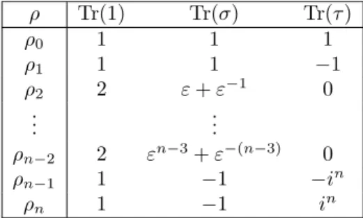
The groupG∆ has order 4n−8, and is often called the binary dihedral group. We label its irre- ducible representations as shown in Table 1. There is a distinguished 2-dimensional representation, the defining representationρnat=ρ2. See [23, 7] for more detailed information.
We will often meet the involution on the set of representations of G∆ which is given by tensor product with the sign representationρ1: on the set of indices{0, . . . , n}, this is the involutionj7→
κ(j) which swaps 0 and 1 andn−1 andn, fixing other values{2, . . . , n−2}. Givenj ∈ {0, . . . , n}, we denote κ(j, k) = κkn(j); this is an involution which is nontrivial when k and n are odd, and trivial otherwise. The special casek= 1 will also be denoted asj =κn(j).
ρ Tr(1) Tr(σ) Tr(τ)
ρ0 1 1 1
ρ1 1 1 −1
ρ2 2 ε+ε−1 0
... ...
ρn−2 2 εn−3+ε−(n−3) 0
ρn−1 1 −1 −in
ρn 1 −1 in
Table 1. Labelling the representations of the groupG∆
The following identities will be useful:
(9) ρ⊗2n−1∼=ρ⊗2n ∼=ρ0, ρn−1⊗ρn∼=ρ1, ρ1⊗ρn−1∼=ρn, ρ1⊗ρn∼=ρn−1, ρ⊗21 ∼=ρ0. 3.2. Young wall pattern and Young walls. We describe here the typeD analogue of the set of labelled partitions used in type A, following [25, 27]. In this section, we only describe the combinatorics; see Appendix A for the representation-theoretic significance of this set.
First we define theYoung wall pattern of type1Dn, the analogue of the (n+ 1)-labelled positive quadrant lattice of typeAn used above. This is the following infinite pattern, consisting of two types of blocks: half-blocks carrying possible labels j ∈ {0,1, n−1, n}, and full blocks carrying possible labels 1< j < n−1:
2 n−2 n−2 2 2
... ...
2 n−2 n−2 2 2
... ...
2 n−2 n−2 2 2
... ...
2 n−2 n−2 2 2
... ...
2 n−2 n−2 2 2
... ...
2 n−2 n−2 2 2
... ...
2 n−2 n−2 2 2
... ...
2 n−2 n−2 2 2
... ...
0 1 n−1 n 0 1
0 1 n−1 n 0 1
0 1 n−1 n 0 1
0 1 n−1 n 0 1
1 0 n n−1
1 0
1 0 n n−1
1 0
1 0 n n−1
1 0
1 0 n n−1
1 0
. . . ...
Next, we define the set ofYoung walls2 of typeDn. A Young wall of typeDn is a subsetY of the infinite Young wall of typeDn, satisfying the following rules.
(YW1) Y contains all grey half-blocks, and a finite number of the white blocks and half-blocks.
(YW2) Y consists of continuous columns of blocks, with no block placed on top of a missing block or half-block.
(YW3) Except for the leftmost column, there are no free positions to the left of any block or half- block. Here the rows of half-blocks are thought of as two parallel rows; only half-blocks of the same orientation have to be present.
1The combinatorics introduced in this section should really be called type ˜D(1)n , but we do not wish to overburden the notation. Also we have reflected the pattern in a vertical axis compared to the pictures of [25, 27].
2In [25, 27], these arrangements are calledproper Young walls. Since we will not meet any other Young wall, we will drop the adjectiveproperfor brevity.
(YW4) A full column is a column with a full block or both half-blocks present at its top; then no two full columns have the same height3.
LetZ∆ denote the set of all Young walls of typeDn. For anyY ∈ Z∆and label j∈ {0, . . . , n}
letwtj(Y) be the number of white half-blocks, respectively blocks, of labelj. These are collected into the multi-weight vectorwt(Y) = (wt0(Y), . . . , wtn(Y)). The total weight ofY is the sum
|Y|= Xn j=0
wtj(Y), and for the formal variablesq0, . . . , qn,
qwt(Y)= Yn j=0
qwtj j(Y).
3.3. Decomposition of C[x, y] and the transformed Young wall pattern. The group G∆
acts on the affine plane C2 via the defining representation ρnat = ρ2. Let S = C[x, y] be the coordinate ring of the plane, then S =⊕m≥0Sm where Sm is themth symmetric power of ρnat, the space of homogeneous polynomials of degreemof the coordinates x, y.
We further decompose
Sm= Mn j=0
Sm[ρj]
into subrepresentations indexed by irreducible representations. We will also use this notation for linear subspaces: forU ⊂Sma linear subspace,U[ρj] =U∩Sm[ρj]. We will call an elementf ∈S degree homogeneous, iff ∈Smfor somem; we call itdegree and weight homogeneous, iff ∈Sm[ρj] for somem, j.
The decomposition of S into G∆-summands can be read off very conveniently from the trans- formed Young wall pattern. The transformation is an affine one, involving a shear: reflect the original Young wall pattern in the linex=y in the plane, translate thenth row bynto the right, and remove the grey triangles of the original pattern. In this way, we get the following picture:
. ..
. . .
2 . . . n−2 n−2 . . . 2 2
2 . . . n−2 n−2 . . . 2 2
2 . . . n−2 n−2 . . . 2 2
2 . . . n−2 n−2 . . . 2 2
0 n−1
n 0
1
0 n−1
n 0
1
1 n−1n 1
0
1 n−1n 1
0
As it can be checked readily, this is a representation of S and its decomposition into G∆- representations. The homogeneous componentsSmare along the antidiagonals. For 1< i < n−1, a full block labelled j below the diagonal, together with its mirror image, correspond to a 2- dimensional representation ρj. For j ∈ {0,1, n−1, n}, a full block labelled j on the diagonal, as well as a half-block labelledj below the diagonal with its mirror image, corresponds to a one- dimensional representation. The dimension ofSm[ρj] is the same as the total number of full blocks labelled j on the mth diagonal in the transformed Young wall pattern, counting mirror images also.
It is easy to translate the conditions (YW1)-(YW4) into the combinatorics of the transformed pattern; see Proposition 3.7 and Remark 3.8 below. Pictures of some small Young walls in the transformed pattern can be found below in Examples 4.5-4.9 below.
3.4. Subspaces and operators. For each non-negative integer m and irreducible representa- tion ρj, consider the space Pm,j of nontrivial G∆-invariant subspaces of minimal dimension in Sm[ρj]. Specifically, ifρj is one-dimensional, then these will be lines, andPm,j is simply the pro- jectivizationPSm[ρj]. Ifρj is two-dimensional, then Pm,j is a closed subvariety of Gr(2, Sm[ρj]).
It is easy to see that in this case also,Pm,j is isomorphic to a projective space.
3This is the properness condition of [25].
More generally, let Grm,j be the space of (r−1)-dimensional projective subspaces of Pm,j. If ρj is one-dimensional, then this is the Grassmannian Gr(r, Sm[ρj]). Whenρj is two-dimensional, thenGrm,j is a closed subvariety of Gr(2r, Sm[ρj]) isomorphic to a Grassmannian of rankr. Clearly G1m,j =Pm,j.
For 0≤j ≤n, we introduce operatorsLj: Gr(S)→Gr(S) on the Grassmannian Gr(S) of all linear subspaces of the vector spaceS as follows: forv∈Gr(S), we set
(1) L0v=v;
(2) L1v=xy·v;
(3) for 1< j < n−1,Ljv=hxj−1·v, yj−1·vi;
(4) Ln−1v= (xn−2−inyn−2)·v;
(5) Lnv= (xn−2+inyn−2)·v.
Sometimes we will use the notation L2 = L2,x +L2,y for the x- and y-component of the op- erator L2, i.e. multiplication with x, respectively y. The operators above restrict to operators L0: Gr(Sm)→Gr(Sm),L1: Gr(Sm)→Gr(Sm+2), Lj: Gr(Sm)→Gr(Sm+j−1) for 1< j < n−1, andLn−1, Ln: Gr(Sm)→Gr(Sm+n−2) on the Grassmannians of the graded piecesSm. To simplify notation, if we do not write the space to which these operators are applied, then application to h1iis meant. So, for example, the symbolL21standing alone denotes the vector subspacehx2y2iof S4, whileL2alone denotes the two-dimensional vector subspacehx, yiofS1. For a linear subspace v of S, the sum P
j∈ILjv denotes the subspace of S generated by the images Ljv. We use the operator notation also for a set of subspaces; the meaning should be clear from the context.
3.5. Cell decompositions of equivariant Grassmannians. We start this section by defining decompositions of the GrassmanniansPm,jof nontrivialG∆-invariant subspaces of minimal dimen- sion inSm[ρj]. Given (m, j), letBm,j denote the set of pairs of non-negative integers (k, l) such thatk+l=m,l≥k, and the block position (k, l) on them-th antidiagonal on or below the main diagonal contains a block or half block of colorj. Here kis the row index,l is the column index, and both of them in a nonnegative integer. It clearly follows from our setup that
dimPm,j=|Bm,j| −1.
Proposition 3.1. Given(m, j), there exists a locally closed stratification Pm,j = G
(k,l)∈Bm,j
Vk,l,j,
which is a standard stratification of the projective spacePm,j into affine spacesVk,l,j of decreasing dimension.
We will callVk,l,j thecellsofPm,j. The decomposition will be defined inductively, based on the following Lemma. Recall thatj7→κ(j) denotes the involution on{0, . . . , n} which swaps 0 and 1 andn−1 andn.
Lemma 3.2. For anyl≥0 and anyj ∈[0, n], we have an injection L1: Pl−2,j→Pl,κ(j).
This map is an isomorphism except in the case when the block or half-block in the bottom row of the transformed Young wall pattern on thel-th antidiagonal has label j, in which case the image has codimension one.
Proof. It is clear that multiplication by L1 induces an injection, so we simply need to check the dimensions. The statement then clearly follows by looking at the transformed Young wall pattern:
multiplication byL1 corresponds to shifting the (l−2)-nd diagonal up by one diagonal step to the l-th diagonal; the number of blocks or half-blocks labelledjis identical, unless the new (half-)block
has labelj, and then the codimension is exactly one.
Remark 3.3. The half-block in the bottom row of the transformed Young wall pattern in the l-th antidiagonal has label j = 0,1 for l ≡0 mod (2n−4) except at (0,0) where only 0 occurs.
Half-blocks labelledj = (n−1), noccur forl≡n−2 mod (2n−4). Forj ∈[2, n−2], there are full blocks labelledj in the bottom row on antidiagonals forl≡j−1 or 2n−3−j mod (2n−4).
Proof of Proposition 3.1. Nontrivial cellsV0,l,j need to be defined exactly when the block or half- block in the bottom row of the transformed Young wall pattern in thel-th antidiagonal has labelj.
In these cases, we set the cells along the bottom row to be V0,l,j=Pl,j\L1Pl−2,κ(j).
Once the cellsV0,k,jalong the bottom row are defined, we define the general cells for all 0≤j ≤n, alll andkby
Vk,k+l,j =Lk1V0,l,κk(j).
What this says is that the cells are shifted up diagonally byL1, taking into account thatL1multi- plies by the sign representation, so shifts the indices by the appropriate power of the involutionκ.
By induction, we obtain a decomposition ofPm,j with the stated properties.
As it is well known, a decomposition of a projectivization of a vector space into affine cells is equivalent to giving a flag in the space itself. This induces a natural decomposition of all higher rank Grassmannians intoSchubert cells, which are known to be affine. Thus our cell decomposition of Pm,j induces cell decompositions of allGrm,j. Since the cells in the first decomposition are indexed by the setBm,j, the cells in the second will be indexed by subsets ofBm,j of sizer. A Schubert cell ofGrm,j corresponding to a subsetS={(k1, l1), . . .(kr, lr)} ⊂Bm,j will consist of those (r−1)- dimensional projective subspaces ofPm,j that intersect Vki,li,j nontrivially for all 1≤i≤r. We will denote the cell corresponding toSin Grm,j byVS,j. We obtain a locally closed decomposition
Grm,j= G
S⊆Bm,j
|S|=r
VS,j.
Occasionally, when it is clear from the context thatSis a subset ofBm,j, we will supress the index j and write justVS for the Schubert cells ofGrm,j.
We will call a Schubert cellmaximal if it intersects the maximal dimensional cell ofPm,j nontriv- ially. Such a cell corresponds to subsetsS⊂Bm,j which contain (kmin, l) where kmin is minimal among the first components of the elements ofBm,j. The intersection withVkmin,l,j of a subspace corresponding to a point in a maximal Schubert cell is an affine subspace ofVkmin,l,j. Conversely, to any affine subspace ofVkmin,l,j, there corresponds a point in a maximal Schubert cell given by the completion of the subspace inPm,j.
For a maximal subsetS, denote byS⊂Bm,jthe set of indices which we get by deleting (kmin, l) fromS. S is empty, if|S|= 1. Define the codimension one projective subspace
Pm,j = G
{(k,l)∈Bm,j:k>kmin}
Vk,l,j ⊂Pm,j =Pm,j\Vkmin,l,j.
For each (r−1)-dimensional subspaceU ⊂Pm,j intersecting the affine spaceVkmin,l,j nontrivially, letU =U∩Pm,j.
Lemma 3.4. The map ω:VS,j →VS,j defined byω(U) =U is a trivial affine fibration with fibre A|Bm,j|−|S|.
We can think of this map as associating to an affine subspace of Vkmin,l,j its set of “ideal points at infinity”. We define the mappingω:VS,j→VS,j as the identity for those index sets and the corresponding cells which are not maximal. In such cases, S =S considered as a subset of Bm,j\ {(kmin, l)}.
Consider the fibreω−1(U) over a pointU ∈VS, which we will also denote byVS|U below. This fibre consists of those subspaces U ⊆ Pm,j which intersect Pm,j in U, i.e. when considered as an affine subspace of Vkmin,l,j, they have U as their set of “points at infinity”. We will denote the set of such subspaces also by Vkmin,l,j/U. This notation means that we take the cosets in Vkmin,l,j of an arbitrary affine subspaceU ⊂Vkmin,l,j withU =Pm,j∩U. The affine structure on Vkmin,l,j descends to an affine structure on Vkmin,l,j/U which does not depend on the particular affine subspaceU whose cosets were taken.
We also need a description of the affine subspaces of the cellsVk,l,j fork > kmin. The relevant Schubert cells in this case are indexed by those subsetsS of Bm,j which contain (k, l) but do not contain any (k′, l′) for k′ < k. Hence, the index setBm,j is first truncated by deleting the pairs