arXiv:1705.06195v3 [math.LO] 5 Feb 2018
D ´ANIEL T. SOUKUP AND LAJOS SOUKUP
Abstract. We explore a general method based on trees of elementary submodels in order to present highly simplified proofs to numerous results in infinite combinatorics. While countable elementary submodels have been employed in such settings already, we significantly broaden this framework by developing the corresponding technique for countably closed models of size continuum. The applications range from various theorems on paradoxical decompositions of the plane, to coloring sparse set systems, results on graph chromatic number and constructions from point-set topology.
Our main purpose is to demonstrate the ease and wide applicability of this method in a form accessible to anyone with a basic background in set theory and logic.
Contents
1. Introduction 1
2. A case study 3
3. Chains versus trees of elementary submodels 5
4. Degrees of disjointness 8
5. Conflict-free colorings 8
6. Clouds above the Continuum Hypothesis 9
7. The chromatic number and connectivity 10
8. Davies-trees from countably closed models 13
9. More on large chromatic number and the subgraph structure 14
10. Coloring topological spaces 15
11. Saturated families 16
12. The weak Freese-Nation property 17
13. Locally countable, countably compact spaces 18
14. Appendix: how to construct sage Davies-trees? 20
15. Final thoughts and acknowledgements 27
References 28
1. Introduction
Solutions to combinatorial problems often follow the same head-on approach: enumerate certain objectives and then inductively meet these goals. Imagine that you are asked to color the points of a topological space with red and blue so that both colors appear on any copy of the Cantor-space in X. So, one lists the Cantor-subspaces and inductively declares one point red and one point blue from each; this idea, due to Bernstein, works perfectly ifX is small i.e. size at most the continuum.
However, for larger spaces, we might run into the following problem: after continuum many steps, we could have accidentally covered some Cantor-subspace with red points only. So, how can we avoid such a roadblock?
Date: February 6, 2018.
2010 Mathematics Subject Classification. 03E05, 03C98, 05C63, 03E35, 54A35.
Key words and phrases. elementary submodels, Davies-tree, clouds, chromatic number, almost disjoint, Bernstein, Cantor, coloring, splendid, countably closed.
1
The methods to meet the goals in the above simple solution scheme vary from problem to problem, however the techniques forfinding the right enumeration of infinitely or uncountably many objectives frequently involve the same idea. In particular, a recurring feature is to write our set of objectivesX as a union of smaller pieceshXα:α < κiso that eachXαresembles the original structureX. This is what we refer to as afiltration. In various situations, we need the filtration to consist of countable sets; in others, we require thatXα⊆ Xβforα < β < κ. In the modern literature, the sequencehXα:α < κiis more than often defined by intersectingX with an increasing chain of countable elementary submodels;
in turn, elementarity allows properties ofX to reflect.
The introduction of elementary submodels to solving combinatorial problems was truly revolution- ary. It provided deeper insight and simplified proofs to otherwise technical results. Nonetheless, note that any setX which is covered by an increasing family of countable sets must have size at mostℵ1, a rather serious limitation even when considering problems arising from the reals. Indeed, this is one of the reasons that the assumption 2ℵ0 =ℵ1, i.e. the Continuum Hypothesis, is so ubiquitous when dealing with uncountable structures.
On the other hand, several results which seemingly require the use of CH can actually be proved without any extra assumptions. So now the question is, how can we define reasonable filtrations by countable sets to cover structures of size bigger thanℵ1? It turns out that one can relax the assumption of the filtration being increasing in a way which still allows many of our usual arguments for chains to go through. This is done by using atree of elementary submodels rather than chains, an idea which we believe originally appeared in a paper of R. O. Davies [4] in the 1960s.
Our first goal will be to present Davies’ technique in detail using his original result and some other simple and, in our opinion, entertaining new applications. However, this will not help in answering the question from the first paragraph. So, we develop the corresponding technique based oncountably closed elementary submodels of size continuum. This allows us to apply Davies’ idea in a much broader context, in particular, to finish Bernstein’s argument for coloring topological spaces. As a general theme, we present simple results answering natural questions from combinatorial set theory; in many cases, our new proofs replace intimidating and technically involved arguments from the literature. We hope to do all this while keeping the paper self contained and, more importantly, accessible to anyone with a basic background in set theory and logic.
Despite its potential, Davies’ method is far from common knowledge even today, though we hope to contribute to changing this. In any case, we are not the first to realize the importance of this method: S. Jackson and D. Mauldin used the same technique to solve the famous Steinhaus tiling problem [20]; also, such filtrations were successfully applied and popularized by D. Milovich [34–37]
under the name of (long)ω1-approximation sequences. In particular, the authors learned about this beautiful technique from Milovich so we owe him a lot.
The structure of our paper is the following: we start by looking at a theorem of W. Sierpinski to provide a mild introduction to elementary submodels in Section 2. Then, in Section 3, we define our main objects of study: the trees of elementary submodels we call Davies-trees; in turn, we present Davies’ original application. We continue with four further (independent) applications of varying difficulty: in Sections 4 and 5, we look at almost disjoint families of countable sets and conflict- free colorings. Next, we present a fascinating result of P. Komj´ath and J. Schmerl in Section 6:
lets say that A ⊂ R2 is a cloud iff every line ℓ through a fixed point a intersects A in a finite set only. Now, how many clouds can cover the plane? We certainly need at least two, but the big surprise is the following: the cardinal arithmetic assumption 2ℵ0 ≤ ℵm is equivalent tom+ 2 clouds coveringR2. In our final application of regular Davies-trees, in Section 7, we will show that any graph with uncountable chromatic number necessarily contains highly connected subgraphs with uncountable chromatic number.
The second part of our paper deals with a new version of Davies’ idea, which we dubbed high Davies-trees. High Davies-trees will be built from countably closed modelsM i.e. A ∈M whenever A is a countable subset ofM. This extra assumption implies thatM has size at leastc but can be extremely useful when considering problems which involve going through all countable subsets of a
structureX. So our goal will be to find a nice filtrationhXα:α < κiof a structureX simultaneously with its countable subsets; whileX can be arbitrary large, eachXα will have size continuum only.
In Section 8, we introduce high Davies-trees precisely. In contrast to regular Davies-trees which exist in ZFC, we do need extra set-theoretic assumptions to construct high Davies-trees: a weak version of GCH and Jensen’s square principle. This construction is carried out only in Section 14 as we would like to focus on applications first. We mention that the results of Section 9, 12 and 13 show that high Davies-trees might not exist in some models of GCH and so extra set theoretic assumptions are necessary to construct these objects.
Now, our main point is that high Davies-trees allow us to provide clear presentation to results which originally had longer and sometimes fairly intimidating proofs. In particular, in Section 10, we prove a strong form of Bernstein’s theorem: any Hausdorff topological spaceX can be colored by continuum many colors so that each color appears on any copy of the Cantor-space in X. Next, in Section 11, we present a new proof that there are saturated almost disjoint families in [κ]ω for any cardinalκ. In our last application in Section 13, we show how to easily construct nice locally countable, countably compact topological spaces of arbitrary large size. All Sections through 9 to 13 can be read independently after Section 8.
Compared to the original statement of the above results, we only require the existence of appropriate high Davies-trees instead of various V = L –like assumptions. This supports our belief that the existence of high Davies-trees can serve as a practical new axiom or blackbox which captures certain useful, but otherwise technical, combinatorial consequences ofV =Lin an easily applicable form. The obvious upside being that anyone can apply Davies-trees without familiarity with the constructible universe or square principles.
Ultimately, Davies-trees will not solve open problems magically; indeed, we mention still unanswered questions in almost each section. But hopefully we managed to demonstrate that Davies-trees do provide an invaluable tool for understanding the role of CH and V =L in certain results, and for a revealing, modern presentation of otherwise technically demanding arguments.
Disclaimer. We need to point out that it is not our intention to give a proper introduction to elementary submodels, with all the prerequisites in logic and set theory, since this has been done in many places already. If this is the first time the kind reader encounters elementary submodels, we recommend the following sources: Chapter III.8 in K. Kunen’s book [32] for classical applications and W. Just, M. Weese [25] for a more lengthy treatment; A. Dow [5] and S. Geschke [15] survey applications of elementary submodels in topology; a paper by the second author [47] gives all the required background in logic with a focus on graph theory. Reading (the first few pages of) any of the above articles will give the additional background for the following sections to anyone with a set theory course already under his or her belt. Nonetheless, an informal introduction is included in Section 2.
We use standard notations following [32]. ZFC denotes the usual Zermelo-Fraenkel axioms of set theory together with the Axiom of Choice. We usecto denote 2ℵ0, the cardinality ofR. CH denotes the Continuum Hypothesis i.e. c = ℵ1. We say that GCH holds (i.e. the generalized Continuum Hypothesis) if 2λ=λ+ for all infiniteλ.
2. A case study
We begin by examining a result of Sierpinski from the 1930s to demonstrate the use of filtrations.
W. Sierpinski produced a myriad of results [45] relating CH to various properties of the reals. Some properties were proved to be equivalent to CH; for others, like the theorem below, Sierpinski could not decide if an actual equivalence holds.
Theorem 2.1( [44]). CH implies thatR2can be covered by countably many rotated graphs of functions i.e. given distinct linesℓi for i < ω through the origin there are sets Ai so that R2 =S{Ai: i < ω}
andAi meets each line perpendicular to ℓi in at most one point.
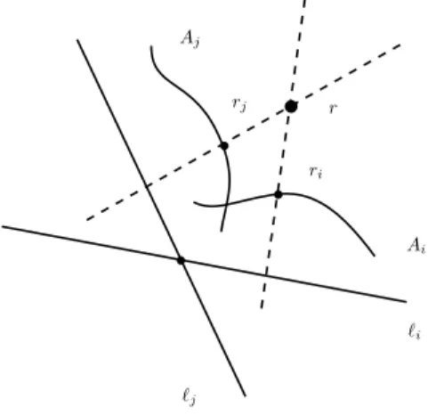
Proof. Fix distinct lines ℓi for i < ω through the origin. Our goal is to find sets Ai so that R2 = S{Ai:i < ω} and ifℓ⊥ℓi (that is,ℓandℓiare perpendicular) then |Ai∩ℓ| ≤1.
If our only goal would be to cover a countable subset R0 = {r0, r1. . .} of R2 first then we can simply letAi={ri}. What if we wish to extend this particular assignment to a cover of a larger set R1 ⊇R0? Given some r∈R1\R0, the only obstacle of puttingr into Ai is that the line ℓ=ℓ(r, i) throughrperpendicular toℓimeets Ai already; we will say thatiis bad forr(see Figure 1).
b b b b
ℓi
ℓj
rj r
ri
Ai Aj
Figure 1. i andj are both bad forr
If alli < ωare bad forrsimultaneously then we are in trouble since there is no way we can extend this cover to includer.
However, note that if i6=j are both bad forr then rcan be constructed from the lines ℓi, ℓj and the points ri, rj (see Figure 1). So constructible points pose the only obstacle for defining further extensions. Hence, in the first step, we should chooseR0so that it is closed under such constructions.
It is easy to see that any setRis contained in a setR∗of size|R|+ω which is closed in the following sense: ifx, y ∈Randi6=j < ω then the intersection ofℓ(x, i) andℓ(y, j) is also inR.
Now the complete proof in detail: using CH, list R2 as {rα:α < ω1} and construct an increasing sequence R0 ⊂R1 ⊂ · · · ⊆ Rα for α < ω1 so that R0 = ({r0})∗, Rα+1 = (Rα∪ {rα})∗ and Rβ = S{Rα:α < β}forβ limit. Note that eachRαis countable and closed in the above sense. Furthermore, S{Rα:α < ω1}=R2.
Next, we define the sets{Ai:i < ω}by first distributingR0trivially as before and then inductively distributing the points in the differences Rα+1 \Rα. Rα+1 \Rα is countable so we can list it as {tn:n < ω}. Given that the points ofRα are assigned to theAi’s already, we will puttn intoA2n or A2n+1. Why is this possible? Because if both 2nand 2n+ 1 are bad for tn then tn is constructible from points inRαand hencetn∈Rα which is a contradiction. This finishes the induction and hence
the proof of the theorem.
One can think of the sequence {Rα : α < ω1} as ascheduling of objectives, where in our current situation an objective is a point inR2 that needs to be covered. We showed that we can easily cover new points given that the setsRαwere closed under constructibility.
Is there any way of knowing, in advance, under what operations exactly our sets need to be closed?
It actually does not matter. Indeed, one can define the closure operation using any countably many functions (and not just this single geometric constructibility) and the closure R∗ of R still has the same size asR (given thatR is infinite). So we can start by saying that{Rα:α < ω1}is a filtration ofR2closed underany conceivable operation and, when time comes in the proof, we will use the fact that eachRαis closed under the particular operations that we are interested in.
Let us make the above argument more precise, and introduce elementary submodels, because the phraseconceivable operation is far from satisfactory.
Let V denote the set theoretic universe and letθ be a cardinal. LetH(θ) denote the collection of sets of hereditary cardinality< θ. H(θ) is actually a set which highly resemblesV. Indeed, all of ZFC
except the power set axiom is satisfied by the model (H(θ),∈); moreover, ifθis large enough then we can take powers of small sets while remaining inH(θ). So, choosing θlarge enough ensures that any argument, with limited iterations of the power set operation, can be carried out inH(θ) instead of the proper model of ZFC.
Definition 2.2. We say that a subset M of H(θ) is an elementary submodel iff for any first order formulaφ with parameters from M is true in(M,∈) iff it is true in(H(θ),∈). We write M ≺H(θ) in this case.
The reason to work with the models (H(θ),∈) is that we cannot express “(M,∈)≺(V,∈)” in first- order set theory (see [21, Theorem 12.7]), but resorting to M ≺H(θ) avoids the use of second-order set theory. Furthermore, for any countable setA ⊆H(θ), there is a countable elementary submodel M ofH(θ) withA⊆M by the downward L¨owenheim-Skolem theorem [32, Theorem I.15.10].
Now, a lot of objects are automatically included in any nonempty M ≺ H(θ): all the natural numbers,ω,ω1orR. Also, note thatM∩R2 is closed under any operation which is defined by a first order formula with parameters fromM.
We need to mention that countable elementary submodels are far from transitive i.e. A∈M does not implyA⊆M in general. However, the following is true:
Fact 2.3. Suppose thatM is a countable elementary submodel of H(θ)andA∈M. IfAis countable thenA⊆M or equivalently, if A\M is nonempty thenA is uncountable.
We present the proof to familiarize the reader with Definition 2.2.
Proof. Suppose that A∈M andAis countable. So H(θ)|=|A| ≤ω. This means that H(θ)|=φ(A) whereφ(x) is the sentence “there is a surjectivef :ω→x”. In turn,M |=φ(A) so we can findf ∈M such that dom(f) = ω and ran(f) = A. We conclude that f(n) ∈ M since n ∈ M for all natural
numbersn∈ω. HenceA= ran(f)⊆M.
Now, how do elementary submodels connect to the closed sets in the proof of Theorem 2.1? Set θ =c+ and take a countable M ≺H(c+) which contains our fixed set of lines {ℓi : i < ω}. We let R=M∩R2and claim thatRis closed under constructibility. Indeed, ifi < ωandx∈R\ℓithen the fact that “ℓis a line throughxorthogonal toℓi” is expressible by a first order formula with parameters inM. HenceM contains as an element a (more precisely, the unique) lineℓ=ℓ(x, i) throughxthat is orthogonal toℓi. So the intersectionℓ(x, i)∩ℓ(y, j) is an element ofM ifx, y∈R. Sinceℓ(x, i)∩ℓ(y, j) is a singleton, Fact 2.3 implies thatℓ(x, i)∩ℓ(y, j)⊆R.
In order to build the filtration{Rα:α < ω1}, we take a continuous, increasing sequence of countable elementary submodelsMα ≺H(c+) and setRα =Mα∩R2. If we make sure thatrα ∈Mα+1 then {Rα:α < ω1}coversR2.
3. Chains versus trees of elementary submodels
In the proof of Theorem 2.1, CH was imperative and Sierpinski already asked if CH was in fact necessary to show Theorem 2.1. The answer came from R. O. Davies [4] who proved that neither CH nor any other extra assumption is necessary beyond ZFC.
We will present his proof now as a way of introducing the main notion of our paper: Davies-trees.
Davies-trees will be special sequences of countable elementary submodels hMα : α < κi covering a structure of sizeκ. Recall that ifκ > ω1 (e.g. we wish to coverR2 while CH fails) then we cannot expect theMα’s to be increasing so what special property can help us out?
The simple idea is that we can always cover a structure of size κ with a continuous chain of elementary submodels of size< κso lets see what happens if we repeat this process and cover each elementary submodel again with chains of smaller submodels, and those submodels with chains of even smaller submodels and so on. . . The following result is a simple version of [34, Lemma 3.17]:
Theorem 3.1. Suppose that κis cardinal, xis a set. Then there is a large enough cardinalθ and a sequence ofhMα:α < κiof elementary submodels of H(θ)so that
(I) |Mα|=ω andx∈Mα for allα < κ, (II) κ⊂S
α<κMα, and
(III) for everyβ < κthere is mβ∈Nand modelsNβ,j≺H(θ)such that x∈Nβ,j for j < mβ and [{Mα:α < β}=[
{Nβ,j :j < mβ}.
We will refer to such a sequence of models as a Davies-tree forκover xin the future (and we will see shortly why they are called trees). The cardinalκwill denote the size of the structures that we deal with (e.g. the size ofR2) while the setxcontains the objects relevant to the particular situation (e.g. a set of lines).
Note that if the sequence hMα : α < κiis increasing then S{Mα : α < β} is also an elementary submodel of H(θ) for each β < κ; as we said already, there is no way to cover a set of size bigger thanω1 with an increasing chain ofcountable sets. Theorem 3.1 says that we can cover by countable elementary submodels and almost maintain the property that the initial segmentsS
{Mα:α < β}are submodels. Indeed, each initial segment is the union of finitely many submodels by condition (III) while these models still contain everything relevant (denoted byxabove) as well.
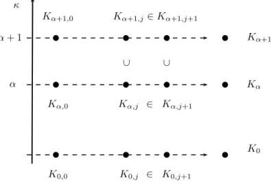
Proof of Theorem 3.1. Letθ be large enough so that κ, x∈H(θ). We recursively construct a tree T of finite sequences of ordinals and elementary submodelsM(a) fora∈T. Let∅ ∈T and letM(∅) be an elementary submodel of sizeκso that
• x∈M(∅),
• κ⊂M(∅).
Suppose that we defined a tree T′ and corresponding models M(a) for a ∈ T′. Fix a ∈ T′ and suppose that M(a) is uncountable. Find a continuous, increasing sequence of elementary submodels hM(a⌢ξ)iξ<ζ so that
• x∈M(a⌢ξ) for allξ < ζ,
• M(a⌢ξ) has size strictly less than M(a), and
• M(a) =S{M(a⌢ξ) :ξ < ζ}.
We extendT′ with{a⌢ξ:ξ < ζ} and iterate this procedure to getT.
M(∅)
M(0) M(1) . . . M(α) . . . M(β) . . .
M(α⌢0) M(α⌢1). . . M(α⌢γ). . .
It is easy to see that this process produces a downwards closed subtreeT of Ord<ω and ifa∈T is a terminal node thenM(a) is countable. Let us well order{M(a) :a∈T is a terminal node} by the lexicographical ordering<lex.
First, note that the order type of<lex isκsince{M(a) :a∈T is a terminal node}has size κand eachM(a) has< κ many<lex-predecessors.
We wish to show that if b∈T is terminal thenS
{M(a) :a<lexb, a∈T is a terminal node} is the union of finitely many submodels containingx. Suppose that|b|=m∈Nand write
Nb,j=[
{M((b↾j−1)⌢ξ) :ξ < b(j−1)}
forj= 1. . . m. It is clear thatNb,jis an elementary submodel as a union of an increasing chain. Also, ifa<lexb thenM(a)⊂Nb,j must hold wherej= min{i≤n:a(i)6=b(i)}. So
[{M(a) :a <lexbis terminal}=[
{Nb,j:j < m}
as desired.
Remarks. Note that this proof shows that ifκ=ℵnthen every initial segment in the lexicographical ordering is the union ofnelementary submodels (the treeT has heightn).
In the future, when working with a sequence of elementary submodels hMα : α < κi, we use the notation
M<β=[
{Mα:α < β}
forβ < κ.
Let us outline now Davies’ result which removes CH from Theorem 2.1:
Theorem 3.2. R2 can be covered by countably many rotated graphs of functions.
Proof. Fix distinct lines ℓi fori < ω through the origin. As before, our goal is to find setsAi so that R2=S{Ai:i < ω}and ifℓ⊥ℓi then|Ai∩ℓ| ≤1.
Let κ=cand take a Davies-treehMα :α < κifor κover{κ,R2, r, ℓi:i < ω} wherer:κ→R2 is onto. So, ifξ∈κ∩Mαthenr(ξ)∈R2∩Mα. In turn,R2⊆S
{Mα:α < κ}.
By induction onβ < κ, we will distribute the points inR2∩M<β among the setsAi while making sure that ifℓ ⊥ℓi then|Ai∩ℓ| ≤1. In a general step, we list the countable set R2∩Mβ\M<β as {tn:n < ω}. Suppose we were able to puttk intoAik fork < nand we considertn.
Recall that M<β can be written as S{Nβ,j : j < mβ} for some finite mβ where each Nβ,j is an elementary submodel containing{κ,R2, r, ℓi:i < ω}. In turn,R2∩M<β is the union ofmβ many sets which are closed under constructibility using the lines{ℓi : i < ω}. This means that there could be at mostmβ manyi∈ω\ {ik :k < n} which is bad fortn i.e. suchiso that the lineℓ(tn, i) through tn which is perpendicular to ℓi already meets Ai. Indeed, otherwise we can find a singlej < mβ and i6=i′∈ω\ {ik:k < n}so that the lineℓ(tn, i) meetsAi∩Nβ,j already andℓ(tn, i′) meetsAi′∩Nβ,j
already. However, this means that tn is constructible from R2∩Nβ,j so tn ∈ Nβ,j as well. This contradictstn∈Mβ\M<β.
So select any in ∈ω\ {ik :k < n} which is not bad for tn and puttn into Ain. This finishes the induction and hence the proof of the theorem.
We will proceed now with various new applications of Davies-trees; our aim is to start with simple proofs and proceed to more involved arguments. However, the next four sections of our paper can be read independently.
Finally, let us mention explicit applications of Davies-trees from the literature that we are aware of (besides Davies’ proof above).
Arguably, the most important application is S. Jackson and R. D. Mauldin’s solution to the Stein- haus tiling problem (see [19] or the survey [20]). In the late 1950s, H. Steinhaus asked if there is a subsetSofR2such that every rotation ofStiles the plane or equivalently,Sintersects every isometric copy of the lattice Z×Z in exactly one point. Jackson and Mauldin provides an affirmative answer;
their ingenious proof elegantly combines deep combinatorial, geometrical and set-theoretical methods (that is, a transfinite induction using Davies-trees). Again, their argument becomes somewhat simpler assuming CH. However, this assumption can be eliminated, as in the Sierpinski-Davies situation, if one uses Davies-trees as a substitute for increasing chains of models. Unfortunately, setting up the appli- cation of Davies-trees in this result is not in the scope of our paper so we chose more straightforward applications.
Last but not least, D. Milovich [34] polished Davies, Jackson and Mauldin’s technique further to prove a very general result in [34, Lemma 3.17] with applications in set-theoretic topology in mind.
In particular, one can guarantee that the Davies-treehMα :α < κihas the additional property that hNα,j : j < mαi,hMβ : β < αi ∈ Mα for all α < κ. This extra hypothesis is rather useful in some situations and will come up later in Section 8 as well. Milovich goes on to apply his technique in further papers concerning various order properties [35, 36] and constructions of Boolean algebras [37].
4. Degrees of disjointness
Let us warm up by proving a simple fact from the theory of almost disjoint set systems. A family of setsAis said to be almost disjoint ifA∩B is finite for allA6=B∈ A. There are two well known measures for disjointness:
Definition 4.1. We say that a family of setsAisd-almost disjointiff|A∩B|< dfor everyA6=B∈ A.
A is essentially disjointiff we can select finiteFA⊂A for eachA∈ A so that{A\FA:A∈ A}is pairwise disjoint.
There are almost disjoint families which are not essentially disjoint; indeed, any uncountable, almost disjoint familyAof infinite subsets of ω witnesses this. However:
Theorem 4.2 ( [27]). Every d-almost disjoint family A of countable sets is essentially disjoint for everyd∈N.
The original and still relatively simple argument uses an induction on|A|. This induction is elimi- nated by the use of Davies-trees.
Proof. Let κ=|A| and take a Davies-treehMα :α < κiforκ over{A, f} where f :κ→ Ais onto.
Note thatA ⊂ S
α<κMα. Also, recall that M<α =S{Nα,j : j < mα} for some mα < ω for each α < κ.
Our goal is to define a mapF onAsuch thatF(A)∈[A]<ωfor eachA∈ Aand{A\F(A) :A∈ A}
is pairwise disjoint.
Let Aα = (A ∩Mα)\M<α and A<α =A ∩M<α. We define F on each Aα independently so fix α < κ.
Observation 4.3. |A∩(SA<α)|< ω for all A∈ Aα.
Proof. Otherwise, there is some j < mα so that A∩S(A ∩Nα,j) is infinite; in particular, we can selecta∈[A∩S
(A ∩Nα,j)]d. Note that S
(A ∩Nα,j)⊂Nα,j since each set inAis countable. Hence a⊂Nα,j and so a∈ Nα,j as well. However,Nα,j |= “there is a unique element of A containinga”
sinceAisd-almost disjoint. SoA∈Nα,j ⊂SM<α by elementarity which contradictsA∈ Aα. Now listAα as{Aα,l:l∈ω}. Let
F(Aα,l) =Aα,l∩ [
A<α∪[
{Aα,k:k < l}
forl < ω. Clearly,F witnesses that Ais essentially disjoint.
In a recent paper, Kojman [26] presents a general framework for finding useful filtrations of ρ- uniformν-almost disjoint families whereρ≥iω(ν). That method is based on Shelah’s Revised GCH and an analysis of density functions.
5. Conflict-free colorings
The study of colorings of set systemsAdates back to the early days of set theory and combinatorics.
Let us say that a mapf :S
A →λis achromatic coloring ofAifff ↾Ais not constant for anyA∈ A.
The chromatic number ofAis the least λso that there is a chromatic coloring ofA. The systematic study of chromatic number problems in infinite setting was initiated by P. Erd˝os and A. Hajnal [8].
this section we will only work with families of infinite sets; note that any essentially disjoint family (and so everyd-almost disjoint as well) has chromatic number 2.
Now, a more restrictive notion of coloring is beingconflict-free: we say thatf :SA →λis conflict- free iff |f−1(ν)∩A| = 1 for some ν < λ for any A ∈ A. That is, any A ∈ A has a color which appears at a unique point ofA. Clearly, a conflict-free coloring is chromatic. We letχCF(A) denote the leastλso that A has a conflict-free coloring. After conflict-free colorings of finite and geometric set systems were studied extensively (see [3, 12, 39, 40]), recently A. Hajnal, I. Juh´asz, L. Soukup and Z. Szentmikl´ossy [18] studied systematically the conflict-free chromatic number of infinite set systems.
We prove the following:
Theorem 5.1. [18, Theorem 5.1] If m, d are natural numbers and A ⊆ [ωm]ω is d-almost disjoint then
χCF(A)≤
(m+ 1)(d−1) + 1 2
+ 2.
(1)
Part of the reason to include this proof here is to demonstrate how Davies-trees forωmcan provide better understanding of such surprising looking results.
Proof. Let A ⊂ [ωm]ω be d-almost disjoint and let hMα:α < ωmi be a Davies-tree for ωm over A.
So each initial segment M<α is the finite union S
j<mNj of elementary submodels. Also, let K = j(m+1)(d−1)+1
2
k+ 2.
We will define eα:ωm∩(Mα\M<α)→K so thate=S
α<ωmeαis a conflict-free coloring ofA.
We start by a simple observation:
Observation 5.2. IfA∈ A ∩(Mα\M<α)then|A∩M<α| ≤m(d−1).
Proof. Indeed, sinceAisd-almost disjoint, anyA∈ Ais uniquely definable fromAand anyd-element subset ofA. SoA ∈Nj ≺H(θ) and|A∩Nj| ≥dwould implyA∈Nj. In turn, |A∩Nj| ≤d−1 for
allj < m.
Now let{An:n∈ω}=A ∩(Mα\M<α) and pick xn∈An\ [
i<n
Ai∪[
{Ak:|Ak∩ {xi:i < n}| ≥d} ∪M<α .
Note that this selection is possible and letX ={xn : n∈ ω}. Clearly, 1 ≤ |X∩An| ≤d+ 1 and xn∈X∩An⊂ {x0. . . , xn}.
We say that a color i < K−1 isbad for An iff there isy 6=z∈An∩(M<α∪ {x0, . . . , xn−1}) such that e(y) =e(z) =i. In other words, i will not witness that the coloring is conflict free on An. We say that a colori < K−1 isgood forAn iff there is a uniquey ∈An∩(M<α∪ {x0, . . . , xn−1}) such thate(y) =i. If there happens to be a good color for An then we simply lete(xn) ={K−1}. This choice ensures thatistill witnesses that the coloringeis conflict-free onAn.
Now, suppose that no colori < K−1 is good forAn. The observation and the fact that|X∩An| ≤ d+ 1 implies that there are at mostj
m(d−1)+d+1 2
k=j
(m+1)(d−1)+1 2
kbad colors forAn. Hence, there is at least one i < K−1 so that no element y ∈ An∩(M<α∪ {x0, . . . , xn−1}) has color i. We let e(xn) =i for such ani < K−1; now,i became a good color forAn. This finishes the induction and the proof of the theorem.
If GCH holds then the above bound is almost sharp ford= 2 or for odd values ofd:
χCF(A)≥
(m+ 1)(d−1) + 1 2
+ 1
for some d-almost disjoint A ⊆ [ωm]ω, and we recommend the reader to look into [18] for a great number of open problems. In particular, Theorem 5.1 gives the bound 4 for m = d = 2; it is not known if equality could hold, even consistently.
6. Clouds above the Continuum Hypothesis
The next application, similarly to Davies’ result, produces a covering of the plane with small sets.
However, this argument makes crucial use of the fact that a set of sizeℵm(form∈N) can be covered by a Davies-tree such that the initial segments are expressed as the union ofmelementary submodels.
Definition 6.1. We say that A ⊂ R2 is a cloud around a point a ∈ R2 iff every line ℓ through a intersectsA in a finite set.
Note that one or two clouds cannot cover the plane; indeed, ifAi is a cloud aroundaifori <2 then the lineℓthrougha0 anda1 intersectsA0∪A1 in a finite set. How about three or more clouds? The answer comes from a truly surprising result of P. Komj´ath and J. H. Schmerl:
Theorem 6.2( [30] and [41]). The following are equivalent for eachm∈N: (1) 2ω≤ ℵm,
(2) R2 is covered by at mostm+ 2clouds.
Moreover,R2 is always covered by countably many clouds.
We only prove (i) implies (ii) and follow Komj´ath’s original argument for CH. The fact that count- ably many clouds always coverR2 can be proved by a simple modification of the proof below.
Proof. Fix m ∈ ω and suppose that the continuum is at most ℵm. In turn, there is a Davies-tree hMα:α <ℵmiforcoverR2 so thatM<α=S{Nα,j:j < m}for everyα <ℵm.
Fix m+ 2 points {ak :k < m+ 2} in R2 in general position (i.e. no three are collinear). Let Lk denote the set of lines throughak and letL=S{Lk :k < m+ 2}. We will define cloudsAk around ak by defining a mapF :L →[R2]<ω such thatF(ℓ)∈[ℓ]<ωand letting
Ak={ak} ∪[
{F(ℓ) :ℓ∈ Lk}
fork < m+ 2. We have to make sure that for everyx∈R2there is ℓ∈ Lso thatx∈F(ℓ).
Now, let Lα = (L ∩Mα)\M<α forα <ℵm. We define F onLα for eachα < ℵm independently so fix anα < ℵm. List Lα\ L′ as {ℓα,i : i < ω} where L′ is the set of m+22
lines determined by {ak:k < m+ 2}. We let
F(ℓα,i) =[
{ℓ∩ℓα,i:ℓ∈ L′∪ {ℓα,i′ :i′ < i}}
fori < ω.
We claim that this definition works: fix a point x∈R2 and we will show that there is ℓ∈ Lwith x∈F(ℓ). Find the uniqueα <ℵm such thatx∈Mα\M<α. It is easy to see that∪L′ is covered by our clouds hence we supposex /∈SL′. Letℓk denote the line throughxandak.
Observation 6.3. |M<α∩ {ℓk:k < m+ 2}| ≤m.
Proof. Suppose that this is not true. Then (by the pigeon hole principle) there is j < m such that
|Nα,j∩ {ℓk:k < m+ 2}| ≥2 and in particular the intersection of any two of these lines, the pointx,
is inNα,j ⊂M<α. This contradicts the minimality ofα.
We achieved that
|{ℓk :k < m+ 2} ∩(Lα\ L′)| ≥2
i.e. there isi′ < i < ω such thatℓα,i′, ℓα,i∈ {ℓk :k < m+ 2}. Hencex∈F(lα,j) is covered by one of the clouds.
7. The chromatic number and connectivity
A graph G is simply a set of vertices V and edges E ⊆ [V]2. Recall that the chromatic number χ(G) of a graphGis the least numberλsuch that the vertices ofGcan be colored byλcolors without monochromatic edges. It is one of the fundamental problems of graph theory how the chromatic number affects the subgraph structure of a graph i.e. is it true that large chromatic number implies that certain graphs (like triangles or 4-cycles) must appear as subgraphs? The first result in this area is most likely J. Mycielski’s construction of triangle free graphs of arbitrary large finite chromatic number [38].
It was discovered quite early that a lot can be said about uncountably chromatic graphs; this line of research was initiated by P. Erd˝os and A. Hajnal in [8]. One of many problems in that paper asked whether uncountable chromatic number implies the existence ofhighly connected uncountably chromatic subgraphs.
A graphGis calledn-connected iff the removal of less thannvertices leavesGconnected. Our aim is to prove P. Komj´ath’s following result:
Theorem 7.1( [28]). Every uncountably chromatic graphG containsn-connected uncountably chro- matic subgraphs for everyn∈N.
Fix a graph G = (V, E), n ∈ ω and consider the set A of all subsets of V inducing maximal n- connected subgraphs of G. We assume thatG has uncountable chromatic number but each A ∈ A induces a countably chromatic subgraph and reach a contradiction.
First,Aessentially coversG:
Lemma 7.2. The graphG↾V \SA is countably chromatic.
Proof. It is proved in [8] that every graph with uncountable chromatic number contains ann-connected
subgraph; hence the lemma follows.
We will follow Komj´ath’s original framework however the use of Davies-trees will make our life significantly easier. We letNG(v) ={w∈V :{v, w} ∈E}forv∈V.
Lemma 7.3. Suppose that G= (V, E)is a graph, the sequencehAξ :ξ < µi coversV with countably chromatic subsets so that
|NG(x)∩A<ξ|< ω for allξ < µ andx∈Aξ\A<ξ
whereA<ξ=S
{Aζ :ζ < ξ}. Thenχ(G)≤ω.
Proof. Suppose that gξ : Aξ → ω witnesses that the chromatic number of Aξ is ≤ ω. We define f : V → ω×ω by defining f ↾ (Aξ\A<ξ) by induction on ξ < µ. If x ∈ Aξ \A<ξ then the first coordinate of f(x) is gξ(x) while the second coordinate of f(x) avoids all the finitely many second coordinates appearing in{f(y) : y ∈ NG(x)∩A<ξ}. It is easy to see that f witnesses that G has
countable chromatic number.
Now, our goal is to enumerateAashAξ :ξ < µiso that the assumptions of Lemma 7.3 are satisfied.
This will imply that the chromatic number ofG↾SAis countable as well which contradicts that G has uncountable chromatic number.
Not so surprisingly, this enumeration will be provided by a Davies-tree but we need a few easy lemmas first.
Observation 7.4. (1) A6⊆A′ for allA6=A′ ∈ A, (2) |A∩A′|< nfor allA6=A′∈ A,
(3) |{A∈ A:a⊂A}| ≤1for all a∈[V]≥n, (4) |NG(x)∩A|< nfor allx∈V \A andA∈ A.
The next claim is fairly simple and describes a situation when we can join n-connected sets.
Claim 7.4.1. Suppose that Ai ⊂ V spans an n-connected subset for each i < n and we can find Y ={yi,k:i, k < n} andX={xk :k < n} distinct points so that
yi,k∈Ai∩NG(xk) for alli, k < n. ThenA=S{Ai :i < n} ∪X isn-connected.
Proof. Let F ∈ [A]<n and note that there is a k < n so that {yi,k, xk : i < n} ∩F = ∅. Thus S{Ai :i < n} ∪ {yi,k, xk :i < n}
\F is connected as Ai\F is connected for all i < n. Finally, if xj ∈A\F thenNG(xj)∩S{Ai:i < n} \F 6=∅so we are done.
Now, we deduce some useful facts about elementary submodels and maximaln-connected sets.
Lemma 7.5. Suppose thatN ≺H(θ)withG∈N and
|NG(x)∩N| ≥n for somex∈V \N. Then x∈A for someA∈ A ∩N.
Proof. Leta∈[NG(x)∩N]n. There is a copy ofKn,ω1 (complete bipartite graph with classes of size nandω1) which containsa∪ {x}; to see this, apply Fact 2.3 toX =T{NG(y) :y∈A}. AsKn,ω1 is n-connected, there must beA∈ Awith a∪ {x} ⊂A as well. Also, there isA′ ∈ A ∩N witha⊂A′ by elementarity; as|A∩A′| ≥nwe haveA=A′ which finishes the proof.
Lemma 7.6. Suppose thatN ≺H(θ)withG∈N and
|NG(x)∩[
(A ∩N)| ≥ω for somex∈V \N. Then x∈A for someA∈ A ∩N.
Proof. Suppose that the conclusion fails; by the previous lemma, we have |NG(x)∩N| < n. In particular, there is sequence of distinctAi∈ A ∩N fori < nso
(NG(x)∩Ai)\N 6=∅ for alli < n(asNG(x)∩Ais finite ifA∈N∩ A).
Thus
N |=∀F ∈[V]<ω∃x∈V \F andyi∈(Ai∩NG(x))\F.
Now, we can find distinct{yi,k:i < n, k < n} andX={xk :k < n} so that yi,k∈Ai∩NG(xk).
Finally,S{Ai:i < n} ∪X isn-connected by Claim 7.4.1 which contradicts the maximality ofAi. Finally, lets finish the proof of Theorem 7.1 by defining this ordering of A. Take a Davies-tree hMα : α < κifor |A| over {G}. In turn, A ⊆ S{Mα : α < κ}. Recall that for all α < κ there is (Nα,j)j<mα so that
M<α=[
{Nα,j :j < mα} withG∈Mα∩Nα,j.
LetA<α=A ∩M<α andAα= (A ∩Mα)\ A<α forα < κ. Well orderAas {Aξ :ξ < µ} so that (1) Aζ ∈ A<α, Aξ∈ A \ A<α impliesζ < ξ and
(2) Aα\ A<α has order type≤ω for allα < κ.
We claim that the above enumeration of A satisfies Lemma 7.3. By the second property of our enumeration and Observation 7.4 (iv), it suffices to show that
|NG(x)∩[
A<α|< ω ifx∈A\SA<α for allA∈ Aα\ A<α andα < κ.
However, asA<α=S{A ∩Nα,j :j < mα}, this should be clear from applying Lemma 7.6 for each of the finitely many modelsNα,j wherej < mα. This finishes the proof of Theorem 7.1.
We note that Komj´ath also proves that every uncountably chromatic subgraph contains an n- connected uncountably chromatic subgraph with minimal degreeω; we were not able to deduce this stronger result with our tools.
It is an open problem whether every uncountably chromatic graph G contains a nonempty ω- connected subgraph [31] (i.e. removing finitely many vertices leaves the graph connected). These infinitely connected subgraphs might only be countable, as demonstrated by
Theorem 7.7( [46]). There is a graph of chromatic numberℵ1and sizecsuch that every uncountable set is separated by a finite set. In particular, everyω-connected subgraph is countable.
8. Davies-trees from countably closed models
In a wide range of problems, we are required to work with countably closed elementary submodels i.e. models which satisfy [M]ω ⊆ M. Recall that it is possible to find countably closed models M with a given parameterx∈ M while the size of M is c. A prime example of applying such models is Arhangelskii’s theorem [1]: every first countable, compact space has size at mostc. In the modern proof of this result [15], a continuousω1-chain of countably closed models, each of sizec, is utilized.
Our main goal in this section is to show that, under certain assumptions, one can construct a sequence of countably closed elementary submodels, each of sizec, which is reminiscent of Davies-trees while the corresponding models cover structures of size> c+; note that this covering would not be possible by an increasing chain of models of sizec.
So, what is it exactly that we aim to show? First, recall that we have been working with the structure (H(θ),∈) so far. However, we will now switch to (H(θ),∈,⊳) where⊳is some (fixed) well- order onH(θ), and use its elementary submodels. We shall see in Section 13 that this can be quite useful e.g. the well order⊳can be used to make uniform choices in a construction of say topological spaces and hence the exact same construction can be reproduced by any elementary submodel with the appropriate parameters.
Now, we say that ahigh Davies-tree forκoverxis a sequencehMα:α < κiof elementary submodels of (H(θ),∈,⊳) for some large enough regularθsuch that
(I) Mαω
⊂Mα,|Mα|=candx∈Mαfor allα < κ, (II)
κω
⊂S
α<κMα, and
(III) for eachβ < κthere are Nβ,j≺H(θ) with [Nβ,j]ω⊂Nβ,j and x∈Nβ,j forj < ω such that [{Mα:α < β}=[
{Nβ,j:j < ω}.
Now, a high Davies-tree is really similar to the Davies-trees we used so far, only that we work with countably closed models of sizec(instead of countable ones) and the initial segmentsM<βare countable unions of such models (instead of finite unions). Furthermore, we require that the models cover
κω
instead ofκitself. This is because our applications typically require to deal with all countable subsets of a large structure.
One can immediately see that (II) implies that κω = κand so high Davies-trees might not exist for some κ. Nonetheless, a very similar tree-argument to the proof of Theorem 3.1 shows that high Davies-trees do exist for the finite successors ofci.e. forκ <c+ω. We will not repeat that proof here but present a significantly stronger result.
As mentioned already, some extra set theoretic assumptions will be necessary to prove the existence of high Davies-trees for cardinals abovec+ω so let us recall two notions. We say thatµ holds for a singularµ iff there is a sequencehCα:α < µ+iso thatCα is a closed and unbounded subset ofαof size< µandCα=α∩Cβ wheneverαis an accumulation point ofCβ. µis known asJensen’s square principle; R. Jensen proved thatµ holds for all uncountableµin the constructible universeL.
Furthermore, a cardinal µ is said to be ω-inaccessible iff νω < µ for all ν < µ. Now, our main theorem is the following:
Theorem 8.1. There is a high Davies-treehMα:α < κifor κoverxwhenever (1) κ=κω, and
(2) µ isω-inaccessible,µω=µ+ andµ holds for allµ withc< µ < κ and cf(µ) =ω.
Moreover, the high Davies-treehMα:α < κican be constructed so that (3) hMα:α < βi ∈Mβ for allβ < κ, and
(4) S{Mα:α < κ} is also a countably closed elementary submodel ofH(θ).
We will say that hMα:α < κiis a sage Davies-tree if it is a high Davies-tree satisfying the extra properties 3. and 4. above. Finally, let us remark that if one only aims to construct high Davies-trees (which are not necessary sage) then slightly weaker assumptions than 1. and 2. suffice; see Theorem 14.2 for further details.
In order to state a rough corollary, recall that 1. and 2. are satisfied by all κ with uncountable cofinality in the constructible universe. Hence:
Corollary 8.2. If V = L then there is a sage Davies-tree for κ over x for any cardinal κ with uncountable cofinality.
Our plan is to postpone the proof of Theorem 8.1 to the appendix in Section 14 because it involves much more work than proving the existence of usual Davies-trees. Indeed, we need a completely different approach than the tree-argument from the proof of Theorem 3.1. Furthermore, we believe that the proof itself gives no extra insight to the use of high Davies-trees in practice.
So instead, we start with applications first in the next couple of sections. We hope to demonstrate that the existence of high/sage Davies-trees can serve as a simple substitute for technically demanding applications ofµ and cardinal arithmetic assumptions.
Some of the presented applications will show that condition (2) in Theorem 8.1 cannot be weakened to say the Generalized Continuum Hypothesis i.e. 2λ =λ+ for all infinite cardinal λ. We will show that consistently, GCH holds and there are no high Davies-trees for any κ above ℵω; we will use a supercompact cardinal for this consistency result (see Corollary 9.2).
Finally, let us point the interested reader to a few related construction schemes which were used to produce similar results: the technique of Jensen-matrices [13], simplified morasses [49] and cofinal Kurepa-families [48, Definition 7.6.11]. In particular, the latter method was used to produce Bernstein- decompositions of topological spaces (see Section 10) and splendid spaces (see Section 13).
9. More on large chromatic number and the subgraph structure
We start with an easy result about large chromatic number and subgraphs, very much in the flavour of Section 7. This result will also demonstrate that high Davies-trees might not exist for anyκ≥ ℵω+1
even if GCH holds.
Let [ℵ0,c+] denote the graph on vertex setU∪V˙ where|U|=ℵ0and|V|=c+, and edges{uv:u∈ U, v∈V}.
Theorem 9.1. Suppose that G is a graph of size λ without copies of [ℵ0,c+]. If there is a high Davies-tree for anyκ≥λoverGthen χ(G)≤c.
The above theorem is a rather weak version of [29, Theorem 3.1]; there GCH and a version of the square principle was assumed to deduce a more general and stronger result.
Proof. Let hMα: α < κi be a high Davies-tree forκ≥λover G. Without loss of generality, we can suppose that the vertex set ofGisλand utilizeλ⊆S{Mα:α < κ}.
Our plan is to define fα : λ∩Mα\M<α → c inductively so that f =S{fα : α < κ} witnesses χ(G)≤c. That is,f is a chromatic coloring: f(u)6=f(v) wheneveruv is an edge ofG.
Suppose we defined colorings fα for α < β such that f<β = S{fα : α < β} is chromatic. List λ∩Mβ\M<β as {vξ : ξ < ν} for someν ≤c and let’s define fβ(vξ) by induction on ξ < ν. Our goal is to choose fβ(vξ) from c\ {fβ(vζ) : ζ < ξ} to make sure that fβ is chromatic, and also that fβ(vξ)6=f<β(u) for anyu ∈λ∩M<β such that uvξ is an edge. If we can do this then f<β∪fβ is chromatic as well.
Our first requirement is easy to meet since we only want to avoid{fβ(vζ) :ζ < ξ}, a set of size<c. The next claim implies that there are not too many edges fromvξ into λ∩M<β:
Claim 9.1.1. Ifv∈λ∩Mβ\M<β then {u∈λ∩M<β:uvis an edge} is countable.
Proof. Recall that M<β =S{Nβ,j : j < ω} so thatG∈Nβ,j and [Nβ,j]ω ⊂Nβ,j. Let N(v) ={u∈ λ:uvis an edge}. IfN(v)∩M<β is uncountable then we can findA∈[N(v)∩Nβ,j]ωfor somej < ω.
SinceA∈Nβ,j, the set B =T{N(u) :u∈A} is also an element of Nβ,j and v ∈B. We claim that
|B|>c; indeed, otherwiseB ⊆Nβ,j and sov∈Nβ,j which contradicts the choice of v. However, any point inA is connected to any point inB which gives a copy of the complete bipartite graph [ℵ0,c+]
inG. This again is a contradiction.
So, we can choose fβ(vξ) and extend our chromatic coloring as desired. In turn, this finishes the induction and the proof of the theorem.
While we do not claim that the existence of a high Davies-tree for κ ≥ λ implies that there are high Davies-trees forλ too, the above proof demonstrates that practically we can work with a high Davies-tree forκas a high Davies-tree forλ.
Corollary 9.2. Consistently, relative to a supercompact cardinal, GCH holds and there are no high Davies-trees for anyκ≥ ℵω+1.
Proof. This will follow from [17, Theorem 4.7]: Consistently, relative to a supercompact cardinal, GCH holds and there is a graphGon vertex setℵω+1of chromatic numberc+ so thatGcontains no copies of [ℵ0,c+].
Now, working in the above model, fixκ≥ ℵω+1, a cardinalθand a well order⊳ofH(θ). LetG∗be the unique⊳-minimal graph on vertex setℵω+1 of chromatic numberc+ so thatG∗contains no copies of [ℵ0,c+]. IfhMα:α < κi is a high Davies-tree forκ≥ ℵω+1 from (H(θ),∈,⊳) then hMα: α < κi must be a high Davies-tree overG∗; indeed,G∗ is uniquely definable fromℵω+1and c+ using ⊳, and these parameters are in each relevant submodel of (H(θ),∈,⊳).
Hence, there are no high Davies-tree for anyκ≥ ℵω+1 in that model by our Theorem 9.1.
10. Coloring topological spaces
Our first application concerns a truly classical result due to F. Bernstein from 1908 [2]: there is a coloring ofRwith two colors such that no uncountable Borel set is monochromatic. In other words, the family of Borel sets inR has chromatic number 2. Indeed, list all the uncountable Borel sets as {Bα :α < c} and inductively pick distinct xβ, yβ ∈Bβ\ {xα, yα : α < β}. This can be done since eachBβ contains a Cantor subspace and so has size continuum. Now any mapf :R→2 that sends {xα:α <c}to 0 and{yα:α <c} to 1 is as desired.
Now, letC(X) denote the set of Cantor subspaces of an arbitrary topological space (X, τ). Can we extend Bernstein’s theorem to general topological spaces? The above simple argument certainly fails if there are more thancmany Cantor subspaces.
Theorem 10.1. Suppose that (X, τ) is a Hausdorff topological space of size κ. If there is a high Davies-tree forκover(X, τ) then there is a coloringf :X →cso that f[C] =cfor anyC∈ C(X).
Let us call such a function f :X →ca Bernstein-decomposition of X. Now, if|X|<c+ωor, more generally,κsatisfies the assumptions of Theorem 8.1 then Bernstein-decompositions forX exist.
Originally, the consistency of “any Hausdorff spaceXhas a Bernstein-decomposition” was originally proved by W. Weiss [50] (see [51] for a survey). For an alternative proof using cofinal Kurepa-families, see [48, Theorem 7.6.31]. Let us also mention that a more general (and more technical) coloring result was achieved in [17, Theorem 3.5] using similar but stronger assumptions to the ones in our Theorem 8.1; it is likely that one can do the same using high Davies-trees. Finally, S. Shelah [42] showed (using a supercompact cardinal) that consistently there is a 0-dim, Hausdorff spaceX of sizeℵω+1 without a Bernstein-decomposition.
Proof. Let hMα : α < κi be a high Davies-tree for κ over X. In turn, X and [X]ω are covered by S{Mα:α < κ}. We letCα=C(X)∩Mα\M<α,Xα=X∩Mα\M<α andX<α=X∩M<α. Claim 10.1.1. Suppose thatC∈ C(X)andC∩X<α is uncountable. Then there is aD∈M<α∩ C(X) such thatD⊆C.
Proof. Indeed, M<α =S{Nα,j : j < ω} and eachNα,j is ω-closed. So there must be an j < ω such thatC∩Nα,j is uncountable. FindA⊆C∩Nα,j which is countable and dense inC∩Nα,j. Note that Amust be an element ofNα,j as well and hence, the uncountable closure ¯AofAis an element ofNα,j
(sinceτ∈Nα,j). Now, we can pickD⊆A¯⊆Csuch thatD∈Nα,j∩ C(X)⊆M<α∩ C(X).
We definefα:Xα→cso thatfα[C] =cfor anyC∈ Cαso thatC∩X<αis countable. This can be done just like Bernstein’s original theorem; indeed let
C∗α={C∩Xα:C∈ Cα,|C∩X<α| ≤ω}.
SCα∗ ⊆ X∩Mα and if Cα∗ 6= ∅ then |SCα∗| = c. Moreover, |Cα∗| ≤ c and Cα∗ is c-uniform i.e. each element has sizec. So, we can use the same induction as Bernstein to findfα.
We claim thatf =S{fα:α < κ} satisfies the requirements. Indeed, suppose that C∈ C(X) and letαbe minimal so that D ⊆C for someD ∈ Cα. Claim 10.1.1 implies that C∩X<α is countable and hencec=fα[D]⊆f[C].
We remark that in the examples preceding this section, Davies-trees were mainly used to find well behaving enumerations of almost disjoint set systems. This is certainly not the case here for the family C(X).
11. Saturated families
The following still open problem stands out in the theory of almost disjoint sets: is there, in ZFC, an infinite almost disjoint family A ⊆[ω]ω so that any B ∈[ω]ω either contains an element fromA or is covered mod finite by a finite subfamily of A. Such families were introduced by Erd˝os and S.
Shelah [10] and are called saturated or completely separable.
Now, in more generality:
Definition 11.1. Let κbe a cardinal andF ⊂ κω
. We say that a familyAisF-saturatedifA ⊂ F and for allF ∈ F either
• A⊂F for someA∈ A, or
• F ⊂∗SA′ for someA′ ∈ A<ω
.
So the completely separable families mentioned at the beginning of the section are exactly the almost disjoint
ωω
-saturated families. Our goal is to prove
Theorem 11.1. If CH holds and there is a high Davies-tree for κ then there is an almost disjoint κω
-saturated family.
First, our theorem gives Baumgartner’s result that CH implies the existence of almost disjoint ℵnω
-saturated families for all finiten(see the remark at Problem 37 in [9]). Second, in [16], similar assumptions (i.e. µand a weak form ofµω=µ+ for cf(µ)< µ) were used to deduce the consistency of “there is an almost disjoint
κω
-saturated family for allκ”.
Proof. Let hMα:α < κi be a high Davies-tree for κ. So, M<α =S
i<ωNα,i for some Nα,i ≺ H(θ) with
Nα,iω
⊂Niα,.
By transfinite recursion onα≤κwe will define familiesAα such that (1) Aα⊆M<α∩[κ]ω is almost disjoint,
(2) Aα⊂ Aβ ifα < β, and
(3) Aα isFα-saturated whereFα=M<α∩ κω
. If we succeed thenAκ is the desired almost disjoint
κω
-saturated family sinceFκ= [κ]ω. In limit steps we can simply take unions so suppose thatAα is defined and we will find Aα+1. Using CH, we can enumerate (Mα\M<α)∩
κω
as {Hξ :ξ < ω1}. By induction on ξ≤ω1, we define familiesBξ such that such that
(i) B0=Aα,|Bξ\ Aα| ≤ω andBη⊂ Bξ ifη < ξ < ω1, (ii) Bξ⊆M<α+1∩[κ]ω is almost disjoint, and
(iii) Bξ is Fα∪ {Hζ :ζ < ξ}
-saturated.