(2008) pp. 31–42
http://www.ektf.hu/ami
Quenching time of solutions for some nonlinear parabolic equations with Dirichlet
boundary condition and a potential
Théodore K. Boni
a, Bernard Y. Diby
baInstitut National Polytechnique Houphouët-Boigny de Yamoussoukro
bUniversité d’Abobo-Adjamé, UFR-SFA Département de Mathématiques et Informatiques
Submitted 9 June 2008; Accepted 15 September 2008
Abstract
In this paper, we address the following initial-boundary value problem
ut(x, t) =Lu(x, t) +r(x)(b−u(x, t))−p in Ω×(0, T), u(x, t) = 0 on ∂Ω×(0, T),
u(x,0) =u0(x)>0 inΩ,
wherep >2,Ωis a bounded domain inRN with smooth boundary∂Ω, Lis an elliptic operator,b=const>0,r∈C1(Ω),supx∈Ωr(x)>0,r(x)is non- negative inΩ,u0 ∈C1(Ω), u0(x)is a nonnegative in Ω, supx∈Ωu0(x)< b.
Under some assumptions, we show that the solution of the above problem quenches in a finite time, and its quenching time goes to that of the solution of the following differential equationα′(t) =r0(b−α(t))−p,t >0,α(0) =M, asM tends tob, whereM = supx∈Ωu0(x)andr0= supx∈Ωr(x).Finally, we give some numerical results to illustrate our analysis.
Keywords: Nonlinear parabolic equation, Dirichlet boundary condition, nu- merical quenching time, quenching
MSC:35B40, 35B50, 35K60, 65M06
1. Introduction
Let Ωbe a bounded domain in RN with smooth boundary ∂Ω. Consider the following initial-boundary value problem for a nonlinear parabolic equation with
31
Dirichlet boundary condition and a potential of the from
ut(x, t) =Lu(x, t) +r(x)(b−u(x, t))−p in Ω×(0, T), (1.1) u(x, t) = 0 on ∂Ω×(0, T), (1.2) u(x,0) =u0(x)>0 in Ω, (1.3) wherep >2,b=const>0,
Lu=
N
X
i,j=1
∂
∂xi
aij(x)∂u
∂xj
,
whereaij: Ω→R, aij ∈C1(Ω), aij=aji,16i, j6N,and there exists a constant C >0such that
N
X
i,j=1
aij(x)ξiξj>Ckξk2 ∀x∈Ω ∀ξ= (ξ1, . . . , ξN)∈RN, wherek.k stands for the Euclidean norm ofRN.
The initial data u0 ∈ C1(Ω), u0(x) is a nonnegative in Ω, supx∈Ωu0(x) < b, r∈C1(Ω), r(x)is nonnegative inΩ,supx∈Ωr(x)>0. Here, (0, T)is the maximal time interval of existence of the solution u of (1.1)–(1.3), and by a solution, we mean the following.
Definition 1.1. A solution of (1.1)–(1.3) is a function u(x, t)continuous in Ω× [0, T), u(x, t)< binΩ×[0, T),and twice continuously differentiable inxand once in tinΩ×(0, T).
The timeT may be finite or infinite. WhenT is infinite, then we say that the solu- tionuexists globally. WhenT is finite, then the solutionudevelops a singularity in a finite time, namely,
t→Tlimku(·, t)k∞=b,
where ku(·, t)k∞ = maxx∈Ω|u(x, t)|. In this last case, we say that the solutionu quenches in a finite time, and the timeT is called the quenching time of the solution u.
Throughout this paper, we suppose that there existsa∈Ωsuch that M = sup
x∈Ω
u0(x) =u0(a) and r0= sup
x∈Ω
r(x) =r(a).
Solutions of nonlinear parabolic equations which quench in a finite time have been the subject of investigations of many authors (see [3–5, 7, 9–15, 18, 21, 22, 24–
26, 28, 29] and the references cited therein). In particular, the above problem has been studied by many authors, and by standard methods based on the maximum principle, local existence, uniqueness, quenching and global existence have been treated (see [7, 23, 24, 29]). In this paper, we are interested in the asymptotic
behavior of the quenching time. Our work was motivated by the paper of Friedman and Lacey in [16], where they have considered the following initial-boundary value problem
ut=ǫ∆u+f(u) in Ω×(0, T), u= 0 on ∂Ω×(0, T), u(x,0) =u0(x)>0 in Ω,
where f(s) is positive, increasing, convex function for nonnegative values of s, R∞
0 ds
f(s) < ∞, ǫ is a positive parameter. The initial data u0(x) is a continuous function in Ω. Under some additional conditions on the initial data, they have proved that the solutionuof the above problem blows up in a finite time, and its blow-up time goes to that of the solution of the following differential equation
α′(t) =f(α(t)), α(0) =M,
as ǫ goes to zero, whereM = supx∈Ωu0(x)(we say that a solution blows up in a finite time if it attains the value infinity in a finite time). Also in [28], Nabongo and Boni have considered the problem (1.1)–(1.3) in the case where the potential r(x) = 1and the operatorLis replaced byǫL. They have obtained a similar result as that found in [16] by Friedman and Lacey. Let us notice that for this kind of problems, other parameters have been taken such that the norm of the initial data (see, for instance [17]) in the case of blow-up problems. In the present paper, we also take the norm of the initial data as parameter and obtain an analogous result using both a modification of Kaplan’s method (see [20]) and a method based on the construction of upper solutions. Our paper is written in the following manner. In the next section, under some conditions, we show that the solutionuof (1.1)–(1.3) quenches in a finite time, and its quenching time goes to that of the solution of a certain differential equation as the norm of the initial data goes to b. Finally, in the last section, we give some numerical results to illustrate our analysis.
2. Quenching times
In this section, under some assumptions, we show that the solutionuof (1.1)–
(1.3) quenches in a finite time, and its quenching time tends to that of the solution of a certain differential equation asM tends tob.
In the introduction of the paper, we have mentioned that there existsa ∈ Ω such thatr0 = supx∈Ωr(x) =r(a)and M = supx∈Ωu0(x) =u0(a). Consider the following eigenvalue problem
−Lψ=λδψ in B(a, δ), (2.1)
ψ= 0 on ∂B(a, δ), ψ >0 in B(a, δ),
where δ >0, such that,B(a, δ) ={x∈RN; kx−ak< δ} ⊂Ω.It is well known that the above eigenvalue problem admits a solution(ψ, λδ)such that0< λδ 6δD2, where D is a positive constant which depends only on the upper bound of the coefficients of the operatorL and the dimensionN. We can normalize ψ so that R
B(a,δ)ψdx= 1.
Now, we are in a position to state the main result of this paper.
Theorem 2.1. Let K be an upper bound of the first derivatives ofu0andr. Sup- pose that supx∈Ωu0(x) =M >0 and letA= (1 +bDK22p)/r0. If
b−M <min{1, A−3/(p+1),(Kdist(a, ∂Ω))3/(p+1)},
then the solutionuof (1.1)–(1.3)quenches in a finite time, and its quenching time T satisfies the following estimates
06T−TM 6 1 r0
1 + A
p+ 1
(b−M)(4p+1)/3+o((b−M)(4p+1)/3), whereTM = (b−Mr0(p+1))p+1 is the quenching time of the solutionα(t) of the differential equation defined as follows
α′(t) =r0(b−α(t))−p, t >0, α(0) =M.
Proof. Since u0 ∈C1(Ω) and r ∈C1(Ω), invoking the mean value theorem and the triangle inequality, we find that
u0(x)>M−(b−M)(p+1)/3 for x∈B(a, δ), r(x)>r0−(b−M)(p+1)/3 for x∈B(a, δ),
whereδ=(b−M)K(p+1)/3.Letw(x, t)be the solution of the following initial-boundary value problem
wt(x, t)−Lw(x, t)−r(x)(b−w(x, t))−p= 0 in B(a, δ)×(0, T∗), (2.2) w(x, t) = 0 on ∂B(a, δ)×(0, T∗),
w(x,0) =u0(x) in B(a, δ),
where (0, T∗) is the maximal time interval of existence of the solution w. By an application of the maximum principle, we see that w is nonnegative in B(a, δ)× (0, T∗), because the initial data is nonnegative inB(a, δ). Introduce the function v(t)defined as follows
v(t) = Z
B(a,δ)
w(x, t)ψ(x)dx for t∈[0, T∗).
Take the derivative of vin tand use (2.2) to obtain v′(t) =
Z
B(a,δ)
ψLwdx+ Z
B(a,δ)
r(x)(b−w)−pψdx for t∈(0, T∗).
Applying Green’s formula, we arrive at v′(t) =
Z
B(a,δ)
wLψdx+ Z
B(a,δ)
r(x)(b−w)−pψdx for t∈(0, T∗).
Due to the fact that r(x)>r0−(b−M)(p+1)/3 > 0 forx∈ B(a, δ), using (2.1) and Jensen’s inequality, we discover that
v′(t)>−λδv(t) + (r0−(b−M)(p+1)/3)(b−v(t))−p. Let us notice that 06v(t)6bfort∈(0, T∗),and
0< λδ 6 D
δ2 = DK2 (b−M)(2p+2)/3. We deduce that
v′(t)>r0(b−v(t))−p
1−(b−M)(p+1)/3 r0
− bDK2(b−v(t))p r0(b−M)(2p+2)/3
for t∈(0, T∗).
Obviously, we have(b−M)(p+1)/36(b−M)(p−2)/3 and
b−v(0)6b−M + (b−M)(p+1)/362(b−M), which implies that
v′(0)>r0(b−v(0))−p(1−A(b−M)(p−2)/3)>0.
We claim that
v′(t)>0 for t∈(0, T∗).
To prove the claim, we argue by contradiction. Indeed, lett0be the firstt∈(0, T∗) such thatv′(t)>0fort∈[0, t0)butv′(t0) = 0.Thus, we havev(t0)>v(0),which implies that
0 =v′(t0)>r0(b−v(0))−p(1−A(b−M)(p−2)/3)>0.
But, this is a contradiction, and the claim is proved. Consequently, we get b−v(t)6b−v(0)62(b−M) for t∈(0, T∗),
and with the help of the above inequalities, we arrive at
v′(t)>r0(b−v(t))−p(1−A(b−M)(p−2)/3) for t∈(0, T∗).
This estimate may be rewritten as follows
(b−v)pdv>r0(1−A(b−M)(p−2)/3)dt for t∈(0, T∗).
Integrate the above inequality over(0, T∗)to obtain (b−v(0))p+1
p+ 1 >r0(1−A(b−M)(p−2)/3)T∗, which implies that
T∗6 (b−M + (b−M)(p+1)/3)p+1 r0(p+ 1)(1−A(b−M)(p−2)/3).
We conclude that w quenches in a finite time because the quantity on the right hand side of the above inequality is finite. On the other hand, by the maximum principle, we have u>0 in Ω×(0, T). Exploiting this estimate, it is easy to see that
ut−Lu−r(x)(1−u)−p>wt−Lw−r(x)(1−w)−p in B(a, δ)×(0, T∗), u>w on ∂B(a, δ)×(0, T∗),
u(x,0)>w(x,0) in B(a, δ),
whereT∗= min{T, T∗}.It follows from the maximum principle that u(x, t)>w(x, t) in B(a, δ)×(0, T∗),
which implies that
T 6T∗6 (b−M + (b−M)(p+1)/3)p+1
r0(p+ 1)(1−A(b−M)(p−2)/3). (2.3) Indeed, suppose that T > T∗. We haveku(·, T∗)k∞ >kw(·, T∗)k∞ =b.But, this is a contradiction because (0, T)is the maximal time interval of existence of the solutionu. Now, settingz(x, t) =α(t)inΩ×[0, T0),it is not hard to see that
zt−Lz−r(x)(1−z)−p= 0 in Ω×(0, T0), z>0 on ∂Ω×(0, T0),
z(x,0)>u0(x) in Ω.
The maximum principle implies that 0 6 u(x, t) 6z(x, t) = α(t) in Ω×(0, T0), whereT0= min{T0, T}.We infer that
T >T0= (b−M)p+1
r0(p+ 1) . (2.4)
Indeed, suppose thatT0> T,which implies thatα(T)>ku(·, T)k∞=b.But, this is a contradiction because(0, T0)is the maximal time interval of existence of the solutionα(t). Apply Taylor’s expansion to obtain
(b−M + (b−M)(p+1)/3)p+1= (b−M)p+1
+(p+ 1)(b−M)(4p+1)/3+o((b−M)(4p+1)/3), 1
1−A(b−M)(p−2)/3 = 1 +A(b−M)(p−2)/3+o((b−M)(p−2)/3).
Use (2.3), (2.4) and the above relations to complete the rest of the proof.
Remark 2.2. Let us notice that the estimates obtained in Theorem 2.1 may be rewritten in the following form
06 T
TM −16(p+ 1 +A)(b−M)(p−2)/3+o((b−M)(p−2)/3).
We deduce thatlimM→b T TM = 1.
3. Numerical results
In this section, we give some computational results to confirm the theory es- tablished in the previous section. We consider the radial symmetric solution of the initial-boundary value problem below
ut= ∆u+ 1
kxk+ 1(1−u)−p in B×(0, T), u= 0 on S×(0, T),
u(x,0) =u0(x) in B,
where B ={x∈RN;kxk<1}, S ={x∈RN;kxk= 1} andu0(x) =Mcos(πkxk2 ) withM ∈(0,1). The above problem may be rewritten in the following form
ut=urr+N−1
r ur+ 1
r+ 1(1−u)−p, r∈(0,1), t∈(0, T), (3.1) ur(0, t) = 0, u(1, t) = 0, t∈(0, T), (3.2)
u(r,0) =ϕ(r), r∈(0,1), (3.3)
where ϕ(r) = Mcos(πr2 ). We start by the construction of some adaptive schemes as follows. Let I be a positive integer and leth= 1/I. Define the grid xi =ih, 0 6 i6I, and approximate the solutionu of (3.1)–(3.3) by the solution Uh(n) = (U0(n), . . . , UI(n))T of the following explicit scheme
U0(n+1)−U0(n)
∆tn =N2U1(n)−2U0(n)
h2 + (1−U0(n))−p, Ui(n+1)−Ui(n)
∆tn
=Ui+1(n)−2Ui(n)+Ui−1(n)
h2 +(N−1)
ih
Ui+1(n)−Ui−1(n) 2h
+ 1
ih+ 1(1−Ui(n))−p, 16i6I−1, UI(n)= 0, Ui(0) =Mcos
ihπ 2
, 06i6I,
where n>0. In order to permit the discrete solution to reproduce the properties of the continuous one when the timet approaches the quenching timeT, we need to adapt the size of the time step so that we take
∆tn= min h2
2N, h2(1− kUh(n)k∞)p+1
with kUh(n)k∞ = sup06i6I|Ui(n)|. Let us notice that the restriction on the time step ensures the nonnegativity of the discrete solution. We also approximate the solutionuof (3.1)–(3.3) by the solutionUh(n) of the implicit scheme below
U0(n+1)−U0(n)
∆tn
=N2U1(n+1)−2U0(n+1)
h2 + (1−U0(n))−p, Ui(n+1)−Ui(n)
∆tn
= Ui+1(n+1)−2Ui(n+1)+Ui−1(n+1)
h2 +(N−1)
ih
Ui+1(n+1)−Ui−1(n+1) 2h
+ 1
ih+ 1(1−Ui(n))−p, 16i6I−1, UI(n+1)= 0, Ui(0)=Mcos
ihπ 2
, 06i6I.
As in the case of the explicit scheme, here, we also choose
∆tn=h2(1− kUh(n)k∞)p+1.
For the above implicit scheme, the existence and nonnegativity of the discrete solution are also guaranteed using standard methods (see, for instance [6]).
We note that
r→0lim ur(r, t)
r =urr(0, t), which implies that
ut(0, t) =N urr(0, t) + (1−u(0, t))−p for t∈(0, T).
This observation has been taken into account in the construction of the above schemes at the first node. We need the following definition.
Definition 3.1. We say that the discrete solutionUh(n) of the explicit scheme or the implicit scheme quenches in a finite time iflimn→∞kUh(n)k∞= 1, and the series P∞
n=0∆tn converges. The quantity P∞
n=0∆tn is called the numerical quenching time of the discrete solution Uh(n).
In the following tables, in rows, we present the numerical quenching times, the numbers of iterations, the CPU times and the orders of the approximations corres- ponding to meshes of 16, 32, 64, 128. We take for the numerical quenching time tn=Pn−1
j=0 ∆tj which is computed at the first time when
∆tn =|tn+1−tn|610−16. The order(s)of the method is computed from
s= log((T4h−T2h)/(T2h−Th))
log 2 .
Numerical experiments
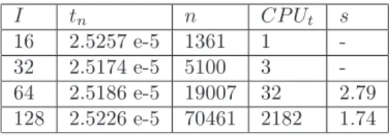
First case: p= 3,N = 2,M = 0.90
Table 1. Numerical quenching times, numbers of iterations, CPU times (seconds) and orders of the approximations obtained with the explicit Euler method.
I tn n CP Ut s
16 2.5257 e-5 1361 1 -
32 2.5174 e-5 5100 3 -
64 2.5186 e-5 19007 32 2.79 128 2.5226 e-5 70461 2182 1.74
Table 2. Numerical quenching times, numbers of iterations, CPU times (seconds) and orders of the approximations obtained with the implicit Euler method.
I tn n CP Ut s
16 2.5258 e-5 1361 1 -
32 2.5174 e-5 5100 6 -
64 2.5186 e-5 19007 155 2.81 128 2.5226 e-5 70461 5534 1.74 Second case: p= 3,N = 2,M = 0.95
Table 3. Numerical quenching times, numbers of iterations, CPU times (seconds) and orders of the approximations obtained with the explicit Euler method.
I tn n CP Ut s
16 1.5725 e-6 1183 1 -
32 1.5657 e-6 4384 3 -
64 1.5642 e-6 16124 44 2.18 128 1.5641 e-6 58833 2373 3.91
Table 4. Numerical quenching times, numbers of iterations, CPU times (seconds) and orders of the approximations obtained with the implicit Euler method.
I tn n CP Ut s
16 1.5725 e-6 1183 1 -
32 1.5657 e-6 4384 4 -
64 1.5642 e-6 16124 103 2.18 128 1.5641 e-6 58833 3366 3.91
Remark 3.2. If we consider the problem (3.1)–(3.3) in the case where the initial dataϕ(r) = 0.9 cos(πr2 )andp= 3,then it is not hard to see that the quenching time of the solution of the differential equation defined in Theorem 2.1 equals 2.5 e-5.
We observe from Tables 1-2 that the numerical quenching time is approximately equal 2.5 e-5. This result has been proved in Theorem 2.1. When the initial data ϕ(r) = 0.95 cos(πr2 )andp= 3,then we find that the quenching time of the solution of the differential equation defined in Theorem 2.1 equals 1.5625 e-5. We discover from Tables 3–4 that the numerical quenching time is approximately equal 1.5625 e-6 which is a result proved in Theorem 2.1.
Acknowledgements. The authors want to thank the anonymous referee for the throughout reading of the manuscript and valuable comment that help us improve the presentation of the paper.
References
[1] Abia, L.M., López-Marcos, J.C., Martínez, J., On the blow-up time conver- gence of semidiscretizations of reaction-diffusion equations,Appl. Numer. Math., 26 (1998) 399–414.
[2] Abia, L.M., López-Marcos, J.C. Martínez, J., Blow-up for semidiscretizations of reaction-diffusion equations,Appl. Numer. Math., 20 (1996) 145–156.
[3] Acker, A., Walter, W., The quenching problem for nonlinear parabolic differ- ential equations, Lecture Notes in Math., Springer-Verlag, New York, 564 (1976) 1–12.
[4] Acker, A., Kawohl, B., Remarks on quenching, Nonl. Anal. TMA, 13 (1989) 53–61.
[5] Bandle, C., Braumer, C.M., Singular perturbation method in a parabolic prob- lem with free boundary,in Proc. BAIL IVth Conference, Boole Press Conf. Ser. 8, Novosibirsk., (1986) 7–14.
[6] Boni, T.K., Extinction for discretizations of some semilinear parabolic equations, C. R. Acad. Sci. Paris, Serie I 333 (2001) 795–800.
[7] Boni, T.K., On quenching of solutions for some semilinear parabolic equations of second order,Bull. Belg. Math. Soc., 7 (2000) 73–95.
[8] Brezis, H., Cazenave, T., Martel, Y., Ramiandrisoa, A., Blow-up ofut = uxx+g(u)revisited,Adv. Diff. Eq., 1 (1996) 73–90.
[9] Chan, C.Y., Lan Ke, Beyond quenching for singular reaction-diffusion problem, Mathematical Methods in the Applied Sciences, 17 (1994) 1–9.
[10] Chan, C.Y., New results in quenching, in Proc. 1st World Congress Nonlinear Anal., (1996) 427–434.
[11] Chan, C.Y., Recent advances in quenching phenomena,Pro. Dynamic Systems and Appl., 2 (1996) 107–113.
[12] Deng, K., Levine, H.A., On the blow-up ofut at quenching,Proc. Amer. Math.
Soc., 106 (1989) 1049–1056.
[13] Deng, K., Xu, M., Quenching for a nonlinear diffusion equation with singular boundary condition,Z. angew. Math. Phys., 50 (1999) 574–584.
[14] Fila, M., Kawohl, B., Levine, H.A., Quenching for quasilinear equations,Comm.
Part. Diff. Equat., 17 (1992) 593–614.
[15] Fila, M., Levine, H.A., Quenching on the boundary, Nonl. Anal. TMA, 21 (1993) 795–802.
[16] Friedman, A., Lacey, A.A., The blow-up time for solutions of nonlinear heat equations with small diffusion,SIAM J. Math. Anal., 18 (1987) 711–721.
[17] Gui, G., Wang, X., Life span of solutions of the Cauchy problem for a nonlinear heat equation,J. Diff. Equat., 115 (1995) 162–172.
[18] Guo, J., On a quenching problem with Robin boundary condition,Nonl. Anal. TMA, 17 (1991) 803–809.
[19] Ishige, K., Yagisita, H., Blow-up problems for a semilinear heat equation with large diffusion,J. Diff. Equat., 212 (2005) 114–128.
[20] Kaplan, S., On the growth of the solutions of quasi-linear parabolic equation, Comm. Appl. Math. Anal., 16 (1963) 305–330.
[21] Kawarada, H., On solutions of initial-boundary problem forut=uxx+ 1/(1−u), Pul. Res. Inst. Math. Sci., 10 (1975) 729–736.
[22] Kirk, C.M., Roberts, C.A., A review of quenching results in the context of non- linear Volterra equations, Dyn. Contin. Discrete Impuls. Syst. Ser. A Math. Anal., 10 (2003) 343–356.
[23] Ladyzenskaya, O.A., Solonnikov, V.A., Ural’ Ceva, N.N., Linear and quasi- linear equations of parabolic type,Trans. Math. Monogr., 23 AMS, Providence, RI, (1968).
[24] Levine, H.A., The phenomenon of quenching: a survey, in Trends In The Theory And Practice Of Nonlinear Analysis,North-Holland, Amsterdam, (1985) 275–286.
[25] Levine, H.A., The quenching of solutions of linear parabolic and hyperbolic equa- tions with nonlinear boundary conditions, SIAM J. Math. Anal., 14 (1983) 1139–
1152.
[26] Levine, H.A., Quenching, nonquenching and beyond quenching for solution of some parabolic equations,Ann. Math. Pura Appl., 155 (1989) 243–260.
[27] Nakagawa, T., Blowing up on the finite difference solution tout=uxx+u2,Appl.
Math. Optim., 2 (1976) 337–350.
[28] Nabongo, D., Boni, T.K., Quenching time for some nonlinear parabolic equations, An. St. Univ. Ovidius Constanta, 16 (2008) 91–106.
[29] Phillips, D., Existence of solution of quenching problems,Appl. Anal., 24 (1987) 253–264.
[30] Protter, M.H., Weinberger, H.F., Maximum principles in differential equations, Prentice Hall, Englewood Cliffs, NJ, (1967).
[31] Shang, Q., Khaliq, A.Q.M., A compound adaptive approach to degenerate non- linear quenching problems,Numer. Meth. Part. Diff. Equat., 15 (1999) 29–47.
[32] Walter, W., Differential-und Integral-Ungleichungen,Springer, Berlin, (1964).
Théodore K. Boni
Institut National Polytechnique Houphouët-Boigny de Yamoussoukro BP 1093 Yamoussoukro, (Côte d’Ivoire)
e-mail: theokboni@yahoo.fr Bernard Y. Diby
Université d’Abobo-Adjamé, UFR-SFA
Département de Mathématiques et Informatiques 02 BP 801 Abidjan 02, (Côte d’Ivoire)
e-mail: ydiby@yahoo.fr