stochastic heat equation with Lévy noise
Carsten Chong∗ Péter Kevei†
Abstract
We examine the almost-sure asymptotics of the solution to the stochastic heat equation driven by a Lévy space-time white noise. When a spatial point is fixed and time tends to infinity, we show that the solution develops unusually high peaks over short time intervals, even in the case of additive noise, which leads to a breakdown of an intuitively expected strong law of large numbers. More precisely, if we normalize the solution by an increasing nonnegative function, we either obtain convergence to 0, or the limit superior and/or inferior will be infinite.
A detailed analysis of the jumps further reveals that the strong law of large numbers can be recovered on discrete sequences of time points increasing to infinity. This leads to a necessary and sufficient condition that depends on the Lévy measure of the noise and the growth and concentration properties of the sequence at the same time. Finally, we show that our results generalize to the stochastic heat equation with a multiplicative nonlinearity that is bounded away from zero and infinity.
AMS 2010 Subject Classifications: 60H15, 60G17, 60F15, 35B40, 60G55
Keywords: additive intermittency; almost-sure asymptotics; integral test; Lévy noise; Poisson noise; stochastic heat equation; stochastic PDE; strong law of large numbers.
1 Introduction
Consider the stochastic heat equation onRd driven by a Lévy space-time white noise ˙Λ, with zero initial condition:
∂tY(t, x) = ∆Y(t, x) +σ(Y(t, x)) ˙Λ(t, x), (t, x)∈(0,∞)×Rd,
Y(0,·) = 0, (1.1)
∗Institut de mathématiques, École Polytechnique Fédérale de Lausanne, Station 8, CH-1015 Lausanne, e-mail:
carsten.chong@epfl.ch
†Bolyai Institute, University of Szeged, Aradi vértanúk tere 1, 6720 Szeged, Hungary, e-mail: kevei@math.u- szeged.hu
1
whereσ:R→(0,∞) is a Lipschitz continuous function that is bounded away from 0 and infinity.
The purpose of this paper is to report on some unexpected asymptotics of the solutionY(t, x), for some fixed spatial pointx∈Rd, as time tends to infinity.
In order to describe the atypical behavior we encounter, let us consider in this introductory part the simplest possible situation where σ ≡ 1 and ˙Λ is a standard Poisson noise, that is, Λ =˙ P∞i=1δ(τi,ηi) is a sum of Dirac delta functions at random space-time points (τi, ηi) that are determined by a standard Poisson point process on [0,∞) ×Rd. In this case, Y(t,·) can be interpreted as the density at time t of a random measure describing particles that are placed according to the point process and perform independentd-dimensional Brownian motions.
As the mild solution Y to (1.1) in this simplified case takes the form Y(t, x) =
Z t 0
Z
Rd
g(t−s, x−y) Λ(ds,dy) =
∞
X
i=1
g(t−τi, x−ηi)1τi<t, (1.2) where
g(t, x) = 1
(4πt)d/2e−|x|
2
4t 1t>0, (t, x)∈[0,∞)×Rd, (1.3) is the heat kernel inddimensions (| · |denotes the Euclidean norm inRd), we immediately see that
E[Y(t, x)] = Z t
0
Z
Rd
g(t−s, x−y) dyds= Z t
0
1 ds=t, (t, x)∈[0,∞)×Rd. (1.4) Hence, one expects to have a strong law of large numbers (SLLN) as t→ ∞in the sense that for fixedx∈Rd, we have
t→∞lim
Y(t, x)
t = 1 a.s.
The starting point of this paper is the observation that the last statement turns out to befalse.
Let us consider without loss of generality the pointx= (0, . . . ,0) and write
Y0(t) =Y(t,0), (1.5)
which is a process with almost surely smooth sample paths by [20, Théorème 2.2.2].
Theorem A. Let f: (0,∞)→(0,∞) be a nondecreasing function, σ ≡1, Y0 be given by (1.5), and Λ˙ be a standard Poisson noise. Then, with probability one, we have
lim sup
t→∞
Y0(t)
f(t) =∞ or lim sup
t→∞
Y0(t) f(t) = 0, according to whether
Z ∞ 1
1
f(t)dt=∞ or
Z ∞ 1
1
f(t)dt <∞.
Furthermore, we almost surely have
lim inf
t→∞
Y0(t) t = 1.
In other words, while the limit inferior follows the expected SLLN, the integral test for the limit superior shows that there is no natural nonrandom normalization that would ensure a nontrivial limit. For example, we have
lim sup
t→∞
Y0(t)
t = lim sup
t→∞
Y0(t)
tlogt =∞ but lim sup
t→∞
Y0(t) t(logt)1.1 = 0
almost surely This kind of phenomenon is common for stochastic processes withinfinite expectation;
see, for instance, [7, Theorem 2] for the case of i.i.d. sums and [4, Theorem III.13] for the case of subordinators (i.e., nonnegative Lévy processes). But it is unusual in our case because Y0 does have a finite expectation by (1.4) (in fact, even a finite variance ifd= 1).
With Gaussian noise, we do not have such irregular behavior but a proper limit theorem:
Theorem B. Suppose that σ ≡ 1 and Λ˙ is a Gaussian space-time white noise in one spatial dimension. Then the following law of the iterated logarithm holds for Y0 from (1.5):
lim sup
t→∞
Y0(t) (2t/π)1/4√
log logt =−lim inf
t→∞
Y0(t) (2t/π)1/4√
log logt = 1 a.s.
In particular, the SLLN holds:
t→∞lim Y0(t)
t = 0 a.s.
This theorem follows easily from the general theory on the growth of Gaussian processes [22].
Although it is known that Y0(t) in the Gaussian case locally looks like a fractional Brownian motion with Hurst parameter 14 (see [16, Theorem 3.3]), we could not find the corresponding global statement specifically for the stochastic heat equation. Hence, we give a short proof of Theorem B at the end of Section 3.4.
Back to the Lévy case, the exact sample path behavior of Y0 is even more complex than described by Theorem A. Our proofs will reveal that the failure of the SLLN for the limit superior is due to the jumps that occur in a short space-time distance to (t, x) = (t,0). However, these problematic jumps that cause the deviation from the SLLN only have a very short impact. In fact, if we only observeY0 on discrete time points, say, at t=tn=np, forn∈Nand some p >0, then we have the following result:
Theorem C. For Y0 from (1.5), if tn=np for some p > d/(d+ 2), we have
n→∞lim Y0(tn)
tn
= 1 a.s., while for 0< p≤d/(d+ 2), we have
lim sup
n→∞
Y0(tn)
tn =∞ and lim inf
n→∞
Y0(tn)
tn = 1 a.s.
So if we sample the solution on a fast sequence (“large p”), those problematic jumps are not visible, and the SLLN does hold true. If the sequence is too slow (“smallp”), they are visible (as in the continuous-time case), and the SLLN fails. Let us make the following observations:
Figure 1: A simulated sample path of t7→Y0(t), n7→Y0(n), n0.5 7→Y0(n0.5), andn0.3 7→Y0(n0.3) under the same realization of a standard Poisson noise in dimensiond= 1. Using Proposition 3.8, we have approximated the contribution of jumps with a distance of more than 5 from x = 0 by the mean. For the plot of t 7→ Y0(t), we have used an equidistant grid of step size 0.01, and have further included for each jump, the time point of the induced local maximum according to Lemma 3.2 in the simulation grid.
(1) The SLLN holds on the sequencetn=n in any dimension.
(2) For any 0< p <1, the SLLN will fail on the sequencetn=np in sufficiently high dimension.
(3) For any dimensiond≥ 1, if we take p ∈ (d/(d+ 2),1), we obtain with tn =np a sequence whose increments ∆tn=tn−tn−1 =np−(n−1)p =O(np−1) converge to 0 as n→ ∞, but on which the SLLN still holds. Together with Theorem A, this means that between infinitely many consecutive points of the sequence tn, which get closer and closer and where Y0 is of ordertn, there are time points whereY0 is significantly larger.
In Figure 1 we see a simulated path of t 7→ Y0(t) for t ∈ [0,200] and its restriction to the sequences n, n0.5, and n0.3, respectively. While unusually large peaks are clearly visible in the plots of t 7→ Y0(t) and n0.3 7→ Y0(n0.3), only small deviations from the linear growth of Y0 are observed on the sequences n and n0.5. This is in agreement with the theoretical considerations above because in dimension 1, the SLLN holds on the sequencenp for allp > 13, while it fails for allp≤ 13 and in continuous time.
A similar dichotomy is also found in Figure 2, which suggests that the averages Y0(n)/n and Y0(n0.5)/n0.5 stabilize at the mean 1 for large values of n, whereas in continuous time or on the
Figure 2: The averagest7→ Y0(t)/t, n7→ Y0(n)/n,n0.5 7→ Y0(n0.5)/n0.5 and n0.3 7→ Y0(n0.3)/n0.3 for the sample path from Figure 1.
sequencen0.3, significant deviations from the mean are repeatedly observed at isolated time points.
Let us interpret these results in a larger context. In the analysis of random fields, many different authors have studied the phenomenon ofintermittency. Originating from the physics literature on turbulence (see [12, Chapter 8]), it refers to the chaotic behavior of a random field that develops unusually high peaks over small areas.
Concerning the stochastic heat equation, it is well known from [2, 11, 16] that the solution to (1.1) driven by a Gaussian space-time white noise in dimension 1 is not intermittent if σ is a bounded function, while it is intermittent if σ has linear growth. Here, intermittency, or more precisely,weak intermittency is mathematically defined as the exponential growth of the moments of the solution. However, the translation of this purely moment-based notion of intermittency to a pathwise description of the exponentially large peaks of the solution, sometimes referred to as physical intermittency, has not been fully resolved yet; see [2, Section 2.4] or [16, Chapter 7.1] for some heuristic arguments. Despite recent results of [18] on the multifractal nature of the space- time peaks of the solution, the exact almost-sure asymptotics of the solution as time tends to infinity, for fixed spatial location, are still unknown. To our best knowledge, only a weak law of large numbers has been proved rigorously for certain initial conditions whenσ is a linear function;
see [3] and, in particular, [1, 10], where much deeper fluctuation results were obtained. Let us also mention that for fixed time, the almost-sure behavior of the solution in space has been resolved in [9, 17].
However, in the case of additive Gaussian noise, Theorem B does reveal the pathwise asymp-
totics of the solution: it obeys the law of the iterated logarithm and is therefore not physically intermittent. But what about the case of Lévy noise? As Theorem A and the last statement in (3) above show, the solution develops high peaks over very short periods of time. So this leads us to the question:
Is the solution Y to (1.1)with Lévy noise physically intermittent?
Certainly not in the sense of exponential growth of the solution because σ is a bounded function (so multiplicative effects cannot build up). But it seems appropriate to say thatY exhibitsadditive physical intermittency. We use the attribute “additive” to describe the fact that the tall peaks of Y0(t) do not arise through a multiplicative cascade of jumps, or the accumulation of past peaks, but rather through the effect of single isolated jumps.
That additive physical intermittency only occurs with jump noise, but not with Gaussian noise, is in line with [6], where we have shown that for the heat equation with multiplicative Lévy noise, weak intermittency occurs on a much larger scale than under Gaussian noise.
Let us mention that a weak (i.e., moment-based) version of additive intermittency has been introduced in a series of papers [13, 14, 15] on superpositions of Ornstein–Uhlenbeck processes.
The term “additive intermittency” itself was coined by Murad S. Taqqu in private communication with the first author discussing the references above.
The remaining paper is organized as follows. In Section 2, we will describe our main results concerning the asymptotic behavior of Y in continuous time as well as on discrete subsequences.
The case of additive Lévy noise will be investigated in Theorems 2.2, 2.3, and 2.4, respectively.
Special cases will be discussed in Corollaries 2.6 and 2.8 and Examples 2.7 and 2.9 in order to illustrate the subtle necessary and sufficient conditions found in these theorems. In Theorems 2.10, 2.11, and 2.12, we then extend the results to the stochastic heat equation with multiplicative noise when the nonlinear functionσ is bounded away from zero and infinity. The proofs will be given in Section 3, where we analyze the “bad” jumps (that could destroy the SLLN) and the “nice” jumps (that behave according to the SLLN) separately in Sections 3.2 and 3.3, before proving the main results in Section 3.4.
Throughout this paper, we useC to denote a strictly positive finite constant whose exact value is not important and may change from line to line.
2 Results
As the Gaussian case is studied separately in Theorem B, we assume from now on that ˙Λ is a Lévy space-time white noise without Gaussian part. More specifically, we suppose that the random measure associated to ˙Λ is given by
Λ(dt,dx) =mdtdx+ Z
R
z(µ−ν)(dt,dx,dz) =m0dtdx+ Z
R
z µ(dt,dx,dz), (2.1) wherem∈Ris the mean of the noise ˙Λ,µis a Poisson random measure on (0,∞)×Rd×Rwhose intensity measureν takes the form ν(dt,dx,dz) = dtdx λ(dz), with a Lévy measureλsatisfying
Z
R
|z|λ(dz)<∞, (2.2)
andm0 =m−R
Rz λ(dz) is thedrift of ˙Λ. In particular, for bounded Borel setsA, Ai ⊆[0,∞)×Rd such that (Ai)i∈N are pairwise disjoint, the random variables (Λ(Ai))i∈N are independent, and we have the Lévy–Khintchine formula
E[eiuΛ(A)] = exp
im0u+ Z
R
(eiuz−1)λ(dz)
Leb(A)
, u∈R,
where Leb denotes the Lebesgue measure on [0,∞)×Rd. In what follows, we always assume that λis not identically zero.
Remark 2.1. Condition (2.2) makes sure that the jumps of the Lévy noise are locally summable.
In fact, ifR[−1,1]|z|pλ(dz) =∞for somep >1, then the sample path t7→Y(t, x), for fixedx∈Rd, is typically unbounded on any nonempty open subset of [0,∞); see [5, Theorem 3.7]. In this case, if the noise has jumps of both signs, we trivially have
lim sup
t→∞
Y0(t)
f(t) =−lim inf
t→∞
Y0(t) f(t) =∞
for any nonnegative nondecreasing functionf, due to the local irregularity of the solution. As the focus of this paper is on the global irregularity of the solution, we will assume (2.2) in all what follows. In particular, by [5, Theorem 3.5], if there exists 0< p <1 such thatR[−1,1]|z|pλ(dz)<∞, thent7→Y(t, x), for fixedx∈Rd, has a continuous modification.
2.1 Additive noise
We first consider the case of additive Lévy noise. It is immediate to see that under the assumption (2.2), the mild solution to (1.1) given by (1.2) is well defined. As in the introduction, we shall fix a spatial point, sayx = (0, . . . ,0), and investigate the behavior of Y0(t) =Y(t,0) ast→ ∞. The following result extends Theorem A to general Lévy noise, assuming a slightly stronger condition than (2.2):
∃ε >0 :mλ(1 +ε) = Z
R
|z|1+ελ(dz)<∞ and
Z 1
−1
|zlogz|λ(dz)<∞. (2.3) Theorem 2.2. Let f: (0,∞)→(0,∞) be a nondecreasing function,σ≡1,Y0 be given by (1.5), and λsatisfy (2.3).
(1) If R1∞1/f(t) dt=∞ andλ((0,∞))>0 (resp., λ((−∞,0))>0), then lim sup
t→∞
Y0(t) f(t) =∞
resp., lim inf
t→∞
Y0(t)
f(t) =−∞
a.s.
(2) Conversely, if R1∞1/f(t) dt <∞, then
t→∞lim Y0(t)
f(t) = 0 a.s.
(3) If λ((0,∞)) = 0 (resp., λ((−∞,0)) = 0), then lim sup
t→∞
Y0(t)
t =m
resp., lim inf
t→∞
Y0(t)
t =m
a.s. (2.4)
Hence, the SLLN fails for any non-Gaussian Lévy noise. Let us remark, however, that the weak law of large numbers does hold true. In particular, there is no (additively) intermittent behavior of the moments of the solution! In the following result, we only consider moments of order less than 1 + 2/dbecause all higher moments are infinite by [6, Theorem 3.1].
Theorem 2.3. Suppose thatσ≡1, thatY0 is given by (1.5), and thatλsatisfies (2.3)with some ε >0. Then for every p∈(0,1 +ε]∩(0,1 + 2/d), we have
Y0(t) t
Lp
−→m as t→ ∞. (2.5)
Next, we continue with our discussion on subsequences. The following theorem extends Theo- rem C to general Lévy noises as well as general sequences and weight functions. Recall the notation
∆tn=tn−tn−1 (with t0= 0) for the increments of tn.
Theorem 2.4. Let f: (0,∞)→(0,∞) be a nondecreasing function,σ≡1,Y0 be given by (1.5), and tn be a nondecreasing sequence tending to infinity. Assume thatλ satisfies (2.3).
(1) If
∞
X
n=1
Z ∞ 0
z f(tn)
2/d
∧∆tn
! z
f(tn)λ(dz) =∞ (2.6) resp.,
∞
X
n=1
Z 0
−∞
|z|
f(tn) 2/d
∧∆tn
! |z|
f(tn)λ(dz) =∞
!
(2.7) andlim infn→∞f(ttn)
n >0, then lim sup
n→∞
Y0(tn) f(tn) =∞
resp., lim inf
n→∞
Y0(tn)
f(tn) =−∞
a.s. (2.8)
(2) Conversely, suppose that the series in (2.6)(resp., (2.7)) is finite. If f is unbounded and
n→∞lim tn
f(tn) =κ∈[0,∞], (2.9)
where κ <∞ when m= 0, then, with probability1, lim sup
n→∞
Y0(tn) f(tn) =κm
resp., lim inf
n→∞
Y0(tn) f(tn) =κm
. (2.10)
Remark 2.5. On the one hand, as we shall explain in Remark 3.11, it is a natural condition to require lim infn→∞f(tn)/tn>0 in the first part of Theorem 2.4. On the other hand, in order that (2.6) or (2.7) hold, the function f must not grow very fast, either. Indeed, if R1∞1/f(t) dt < ∞, thenP∞n=1∆tn/f(tn)<∞ by Riemann-sum approximation, so (2.6) and (2.7) cannot be true (in agreement with part (2) of Theorem 2.2). Typical functions that we have in mind are f(t) =tor f(t) =tlog+t(where log+(t) = log(e+t)).
Theorem 2.4 has a number of surprising consequences. We shall explain them as well as the conditions (2.6) and (2.7) through a series of corollaries and examples.
If we bound the minimum in (2.6) (resp., (2.7)) by the first term, we immediately obtain the following result:
Corollary 2.6. If Z ∞
0
|z|1+2/dλ(dz)<∞
resp., Z 0
−∞
|z|1+2/dλ(dz)<∞
and
∞
X
n=1
1
f(tn)1+2/d <∞,
(2.11)
then the series in (2.6) (resp., (2.7)) is finite.
Upon takingf(x) =x and tn=np, we immediately obtain the first statement of Theorem C.
Observe that (2.11) separates the complicated expressions in (2.6) and (2.7) into a simple size condition on the jumps and a simplegrowth condition on the sequence tn. But in general, for the SLLN to hold, we neither need (1 + 2/d)-moments, nor does the sequence have to grow fast.
We write an∼bnif limn→∞an/bn= 1 andan≈bnif there are constants C1, C2∈(0,∞) such thatan/bn∈[C1, C2] for large values ofn. The same notation is also used for continuous variables.
Example 2.7 (Condition (2.11) is not necessary). Neither the condition on the jumps nor the condition ontn in (2.11) is necessary.
(1) Consider the sequencetn=np withp >0 andf(t) =t. Then ∆tn∼pnp−1. Furthermore, Z ∞
0
z np
2/d
∧np−1
! z
np λ(dz) =
Z np+(p−1)d/2 0
z1+2/d
np(1+2/d) λ(dz) + Z ∞
np+(p−1)d/2
z nλ(dz), where we use the convention Rab = R(a,b]. Summing over n ∈ N and changing integral and summation, we obtain
Z ∞ 0
X
np+(p−1)d/2≥z
z1+2/d
np(1+2/d) + X
np+(p−1)d/2<z
z n
λ(dz). (2.12)
The second sum in the integral above is finite only if p+ (p−1)d/2 > 0, or equivalently p > d/(d+ 2). Then the first sum in the integral is ≈ z1+2/dz(1−p(1+2/d))/(p+(p−1)d/2) = z, while the second sum is≈zlog+(z)1z>1. Hence, the expression in (2.12) is finite if and only
if R0∞zlog+(z)λ(dz) < ∞, which is always true by (2.3). The same argument obviously applies to the negative jumps as well. Thus, under (2.3), and if λ((0,∞)) > 0 (resp., λ((−∞,0))>0), the series in (2.6) (resp., (2.7)) is finite for the sequencetn=np if and only ifp > d/(d+ 2). This shows that the first part in (2.11) is not a necessary condition.
(2) An easy counterexample also shows that the second condition in (2.11) is not necessary.
Consider the sequence (tn)n∈N that visits each n∈Nexactlyn times, that is,
t1= 1, t2 =t3 = 2, t4 =t5=t6= 3, t7 =t8 =t9 =t10= 4 etc. (2.13) Then, from the SLLN on the sequencen, we derive
n→∞lim Y0(tn)
tn = lim
n→∞
Y0(n) n =m.
But we have
∞
X
n=1
1 t1+2/dn
=
∞
X
n=1
n n1+2/d =
∞
X
n=1
1 n2/d, which is infinite ford≥2.
In (2.13), we have seen a sequence tn on which the SLLN holds although it grows relatively slowly. Indeed, we havetn=O(√
n) and the SLLN fails on the sequence√
nifd≥2; see the first part in Example 2.7. So the growth of a sequencetn does not fully determine whether the SLLN holds or not. In fact, we have found an example of two sequences (sn)n∈N and (tn)n∈N where we have sn ≥ tn for all n ∈ N, but the SLLN only holds on (tn)n∈N and not on (sn)n∈N. Hence, in order to determine whether the SLLN holds or not on a given sequence, we have to take into account itsclustering behavior, in addition to its speed. This is why the increments ∆tnenter the conditions (2.6) and (2.7). The following criterion is an improvement of Corollary 2.6.
Corollary 2.8. Suppose that Z ∞
0
|z|1+2/dλ(dz)<∞
resp., Z 0
−∞
|z|1+2/dλ(dz)<∞
(2.14) and that λ((0,∞))6= 0 (resp., λ((−∞,0))6= 0). Then the series in (2.6) (resp., (2.7)) converges if and only if
∞
X
n=1
f(tn)−2/d∧∆tn
f(tn) <∞. (2.15)
In particular, if mλ(1 + 2/d)<∞ and λ6= 0, the SLLN holds on tn if and only if tn satisfies (2.15)with f(t) =t.
Proof. We write the left-hand side of (2.6) as
∞
X
n=1
Z f(tn)(∆tn)d/2 0
z1+2/d
f(tn)1+2/dλ(dz) + Z ∞
f(tn)(∆tn)d/2
z∆tn f(tn)λ(dz)
! ,
and split this sum into two parts,I1 and I2, according to whethern belongs to
I1 ={n∈N: ∆tn≤f(tn)−2/d} or I2 ={n∈N: ∆tn> f(tn)−2/d}.
Then by (2.3) and (2.15), I1≤ X
n∈I1
(f(tn)(∆tn)d/2)2/d f(tn)1+2/d
Z 1 0
z λ(dz) + ∆tn
f(tn) Z ∞
0
z λ(dz)
!
≤2 Z ∞
0
z λ(dz) X
n∈I1
∆tn
f(tn) <∞, and
I2 ≤ X
n∈I2
1 f(tn)1+2/d
Z ∞ 0
z1+2/dλ(dz) + Z ∞
0
z(z/f(tn))2/d f(tn) λ(dz)
!
≤2 Z ∞
0
z1+2/dλ(dz) X
n∈I2
1
f(tn)1+2/d <∞,
which shows one direction in (2.15). The other direction follows from I1 ≥ X
n∈I1
Z f(tn)(∆tn)d/2 0
z1+2/d∆tn
f(tn) λ(dz) + Z ∞
f(tn)(∆tn)d/2
z∆tn
f(tn)λ(dz)
!
≥ X
n∈I1
∆tn f(tn)
Z ∞ 0
(z∧z1+2/d)λ(dz) and
I2≥ X
n∈I2
Z f(tn)(∆tn)d/2 0
z1+2/d
f(tn)1+2/dλ(dz) + Z ∞
f(tn)(∆tn)d/2
z
f(tn)1+2/dλ(dz)
!
≥ X
n∈I2
1 f(tn)1+2/d
Z ∞ 0
(z∧z1+2/d)λ(dz).
An analogous argument applies to (2.7).
Is it possible to separate (2.6) and (2.7) into a condition on the Lévy measureλand a condition on the sequence tn? And is it possible to determine whether the SLLN holds or not by only looking at the sequence tn, without assuming a finite (1 + 2/d)-moment as in Corollary 2.8, but only assuming a finite first moment (or a finite (1 +ε)-moment as in (2.3))? The answer isno, in both cases.
Example 2.9 (Conditions (2.6) and (2.7) are not separable). Consider f(t) = t and the sequence tn = (n(log+n)1+θ)d/(d+2) for some θ > 0 (in particular, (2.15) is satisfied). By the mean-value theorem, it is not difficult to see that
∆tn≈n−2/(d+2)(log+n)(1+θ)d/(d+2), ∆tn tn
≈n−1, tn(∆tn)d/2 ≈(log+n)(1+θ)d/2. (2.16)
Next, let us take the Lévy measure
λ(dz) =z−1−α1[1,∞)(z) dz
for someα ∈(1,1 + 2/d). In particular, ifα∈(1,2), the Lévy noise will have the same jumps of size larger than 1 as anα-stable noise. It is easy to verify that the chosen Lévy measure has finite moments up to orderα (but not includingα) so that (2.3) is satisfied, but (2.14) is not.
In this set-up, the series in (2.6) becomes
∞
X
n=1
Z tn(∆tn)d/2 1
z tn
1+2/d
z−1−αdz+
∞
X
n=1
Z ∞ tn(∆tn)d/2
z∆tn
tn
z−1−αdz. (2.17) Regarding the first sum, (2.16) implies that
Z tn(∆tn)d/2 1
z tn
1+2/d
z−1−αdz≈ 1 n(log+n)1+θ
Z (log+n)(1+θ)d/2 1
z2/d−αdz
≈ (log+n)(1+2/d−α)(1+θ)d/2
n(log+n)1+θ , which in turn shows that the first sum in (2.17) converges if and only if
α >1 + 2
d(1 +θ). (2.18)
The same holds for the second sum in (2.17) because by (2.16), Z ∞
tn(∆tn)d/2
z∆tn tn
z−1−αdz≈n−1 Z ∞
(log+n)(1+θ)d/2
z−αdz≈n−1(log+n)(1−α)(1+θ)d/2.
Altogether, the series in (2.6) converges if and only if (2.18) holds, which involvesα(a parameter of the noise) andθ(a parameter of tn) at the same time.
Corollary 2.8 and Example 2.9 also show the following peculiar fact. If the jumps of Λ have a finite (1 + 2/d)-moment, then whether we have the SLLN on (tn)n∈N or not, only depends on this sequence itself; the details of the Lévy measure (i.e., the distribution of the jumps) do not matter.
So if Λ has both positive and negative jumps, we either have the SLLN on tn, or we see peaks in both directions, in the sense that the limit superior/inferior ofY0(tn)/tn is±∞.
But for noises with an infinite (1 + 2/d)-moment, and again jumps of both signs, we may have a sequencetnon which the SLLN (withf(t) =t) only fails in one direction. That is, we see peaks, for instance, for the limit superior, but then have convergence to the mean for the limit inferior.
By Theorem 2.2, this does not happen in continuous time: if we have both positive and negative jumps, we see both positive and negative peaks.
2.2 Multiplicative noise with bounded nonlinearity
Without much additional effort, we can generalize Theorems 2.2, 2.3, and 2.4 to the stochastic heat equation with a bounded multiplicative nonlinearity. Consider (1.1) where σ:R → R is a
globally Lipschitz function that is bounded and bounded away from 0, that is, there are constants k1, k2 >0 such that
k1< σ(x)< k2, x∈R. (2.19)
It is well known from [20, Théorème 1.2.1] that if λ satisfies (2.2) (in particular, if (2.3) holds), and ˙Λ has no Gaussian part, then (1.1) has a unique mild solution Y, that is, there is a unique predictable processY that satisfies the integral equation
Y(t, x) = Z t
0
Z
Rd
g(t−s, x−y)σ(Y(s, y)) Λ(ds,dy).
We continue to writeY0(t) =Y(t,0).
Theorem 2.10. Suppose that f: (0,∞)→ (0,∞) is nondecreasing and that σ:R→ R is Lips- chitz continuous and satisfies (2.19). Furthermore, assume that (2.3)holds.
(1) Part (1) and part (2) of Theorem 2.2 remain valid.
(2) Part (3) of Theorem 2.2 remains valid if we replace (2.4) by lim sup
t→∞
Y0(t) t <∞
resp. lim inf
t→∞
Y0(t)
t >−∞
a.s.
Theorem 2.11. Suppose thatλand p are as in Theorem 2.3 and that σ is Lipschitz continuous and satisfies (2.19). Then, instead of (2.5), we have
lim sup
t→∞ E
Y0(t) t
p
<∞.
Theorem 2.12. Suppose that f, (tn)n∈N, andλ satisfy the same hypotheses as in Theorem 2.4.
Moreover, let σ be Lipschitz continuous with the property (2.19).
(1) Part (1) of Theorem 2.4 remains valid.
(2) Part (2) of Theorem 2.4 remains valid if κ <∞ in (2.9), and if (2.10) is replaced by lim sup
n→∞
Y0(tn) f(tn) <∞
resp. lim inf
n→∞
Y0(tn)
f(tn) >−∞
a.s.
Remark 2.13. If (2.19) is violated, then we no longer expect the last three results to hold. For example, if we consider the parabolic Anderson model with Lévy noise, that is, (1.1) withσ(x) =x (and a nonzero initial condition), it is believed that the solution develops exponentially large peaks as time tends to infinity (multiplicative intermittency). While the moments of the solution indeed grow exponentially fast as shown in [6], its pathwise asymptotic behavior is yet unknown. Only for a related model, where the noise ˙Λ is obtained by averaging a standard Poisson noise over a unit ball in space (so that the resulting noise is white in time but has a smooth covariance in space), it was proved in [8] for delta initial conditions that t7→R
RdY(t, x) dx has exponential growth int almost surely.
3 Proofs
In the following, we denote the points of the Poisson random measureµby (τi, ηi, ζi)i∈N and refer toτi,ηi, andζias thejump time,jump location, andjump size, respectively. For the fixed reference pointx= (0, . . . ,0) and some givent >0, we shall say that (τi, ηi, ζi) withτi ≤tis a
• recent (resp.,old) jump ift−τi ≤1 (resp., t−τi >1);
• close (resp.,far) jump if|ηi| ≤1 (resp., |ηi|>1);
• small (resp., large) jump if|ζi| ≤1 (resp., |ζi|>1).
A key to the proofs below is to decompose Y0(t) into a contribution of the recent close jumps and a contribution by all other jumps. That is, by (1.2) and (2.1), we have
Y0(t) = Z t
0
Z
Rd
g(t−s, y)Λ(ds,dy) =X
τi≤t
g(t−τi, ηi)ζi+m0t=:Y1(t) +Y2(t), where
Y1(t) = X
τi∈(t−1,t],|ηi|≤1
g(t−τi, ηi)ζi, Y2(t) =m0t+ X
τi≤t−1 or|ηi|>1
g(t−τi, ηi)ζi. (3.1)
We also consider the decomposition Y1 = Y1+ +Y1−, where Y1+ (resp., Y1−) only contains the positive (resp., negative) jumps in the definition ofY1 in (3.1).
3.1 Some technical lemmas and notation
We begin with four simple lemmas: a tail and a large deviation estimate for Poisson random variables, two elementary results for the heat kernel, and one simple result from analysis.
Lemma 3.1. Suppose that Xλ follows a Poisson distribution with parameterλ >0.
(1) For everyn∈N, we have
P(Xλ≥n)≤ λn n!. (2) If x≥aλ, where a >1, then
P(Xλ≥x)≤e−x(loga−1+1a). (3.2) In particular, fora= 2, we have
P(Xλ ≥x)≤e−δ0x, where δ0 = log 2−1/2≈0.193.
Proof. By Taylor’s theorem, there existsθ∈[0,1] such that P(Xλ ≥n) =e−λ
∞
X
k=n
λk
k! =e−λ eλ−
n−1
X
k=0
λk k!
!
=e−λeθλλn n! ≤ λn
n!,
which proves the first claim. For the second claim, we have by Markov’s inequality for anyu >0, P(Xλ≥x)≤P(euXλ ≥eux)≤e−uxE[euXλ] =e−(ux+λ−λeu).
Choosingu= log(x/λ), we obtain
P(Xλ ≥x)≤e−x(logxλ−1+λx).
Since λ/x ∈ (0,1/a] and the function u 7→ logu−1−1 +u is decreasing on (0,1), the statement follows.
Lemma 3.2. Let g be the heat kernel given in (1.3).
(1) For fixedx ∈Rd, g(t, x) is increasing on [0,|x|2/(2d)], decreasing on [|x|2/(2d),∞), and its maximum is
g(|x|2/(2d), x) = d
2πe d/2
|x|−d. (3.3)
(2) The time derivative of g is given by
∂tg(t, x) = e−|x|
2 4t
π|x|2
t −2πd
(4πt)d/2+1 , (t, x)∈(0,∞)×Rd. (3.4) There exists a finite constantC >0 such that for all (t, x)∈(0,∞)×Rd,
|∂tg(t, x)| ≤
(C|x|−d−2 if |x|2 >2dt,
Ct−d/2−1 if |x|2 ≤2dt. (3.5) Proof. Both (3.3) and (3.4) follow from standard analysis. The second half of (3.5) follows easily from (3.4). For the first half, using the inequality supy>0e−yyd/2+2 <∞, we have for |x|2 ≥2dt that
|∂tg(t, x)| ≤e−|x|
2 4t π|x|2
t (4πt)−d/2−1=Ce−|x|
2 4t |x|2
4t
!d/2+2
|x|−d−2≤C|x|−d−2.
Lemma 3.3. For every ε >0, there existsδ =δ(ε)>0 such that
g(t+s, x)≥(1−ε)g(t, x) (3.6)
holds under either of the two following conditions:
(1) s, t >0,x∈Rd, ands/t≤δ;
(2) s, t >0,x∈Rd, |x|>1, and s < δ.
Proof. By definition, we have g(t+s, x)≥(1−ε)g(t, x) if and only if e
|x|2
4 (1t−t+s1 )≥(1−ε)
1 +s t
d/2
.
The left-hand side is greater than or equal to 1, since the exponent is positive. Therefore, the inequality is true if the right-hand side is less than or equal to 1. Under condition (1), we have s/t∈(0, δ), so it suffices to make sure that
(1−ε)(1 +δ)d/2≤1.
This holds if we chooseδ≤δ1 = (1−ε)−2/d−1.
In case (2), if t > 1/(2d), we have s/t < 2dδ, so by (1), (3.6) holds if s ≤ δ2 = δ1/(2d). If 0< t≤1/(2d), then |x|>1 implies that
g(t, x) g(t+s, x) =
1 +s
t d/2
e−
|x|2s 4t(t+s) ≤
1 +s
t d/2
e−4t(t+s)s .
For fixeds >0, elementary calculus shows that the term on the right-hand side reaches its unique maximum at
t=
√d2s2+ 1−ds+ 1
2d ≥ 1
2d. Hence, fort <1/(2d) and s < δ2, we obtain that
g(t, x)
g(t+s, x) ≤(1 + 2ds)d/2e− d
2s
2ds+1 ≤(1 + 2dδ2)d/2= (1−ε)−1. The claim now follows by takingδ(ε) =δ1∧δ2 =δ2.
Lemma 3.4. Suppose that f: (0,∞)→(0,∞) is nondecreasing.
(1) If R1∞1/f(t) dt <∞, then
t→∞lim f(t)
t =∞.
(2) If R1∞1/f(t) dt=∞, then
Z ∞ 1
1
f(t)∨tdt=∞. (3.7)
Proof. For (1), if we had lim inft→∞f(t)/t < ∞, then there would be a sequence (an)n∈N with a1 = 1 and increasing to infinity such that f(an) ≤ Can for all n ∈ N. Then, because f is nondecreasing,
Z ∞ 1
1 f(t)dt≥
∞
X
n=1
Z an+1
an
1
f(an+1)dt≥
∞
X
n=1
an+1−an
Can+1 =∞,
which would be a contradiction, provided we can prove the last equality.
For any fixed m∈N, we have
∞
X
n=m
an+1−an
an+1 ≥
N−1
X
n=m
an+1−an
an+1 ≥
N−1
X
n=m
an+1−an
aN = aN −am
aN −→1, asN → ∞, so the infinite sum diverges as claimed.
For (2), suppose that the integral in (3.7) were finite. As f(t)∨tis nondecreasing, by the first part of the lemma,
t→∞lim
f(t)∨t
t =∞,
which would implyf(t)≥t for large values oft, and thus R1∞1/f(t) dt <∞, a contradiction.
Finally, let us introduce some notation: B(r) ={x∈Rd:|x| ≤r}denotes the ball with radius r >0, and B(r1, r2) ={x∈Rd:r1 ≤ |x| ≤r2} for 0 < r1 < r2. Furthermore,vd is the volume of B(1), and λ(x) =λ((x,∞)). For r >0 and 0≤r1< r2, we write
U(r) =
(y, z) : z
|y|d > r,|y| ≤1
, U(r1, r2) =
(y, z) : z
|y|d ∈[r1, r2],|y| ≤1
. (3.8) If`is the Lebesgue measure on Rd, then short calculation gives
`⊗λ(U(r1, r2)) =vd
Z ∞ 0
z r1
∧1
− z
r2
∧1
λ(dz)
=vd
(r−11 −r2−1) Z r1
0
z λ(dz) + Z r2
r1
1− z
r2
λ(dz)
=ψ(r1)−ψ(r2),
(3.9)
where
ψ(r) =vd 1
r Z r
0
z λ(dz) +λ(r)
= vd r
Z r 0
λ(z) dz. (3.10)
We also use the simpler bound
`⊗λ(U(r)) =vd
Z ∞ 0
z r ∧1
λ(dz)≤ vd
r Z ∞
0
z λ(dz). (3.11)
3.2 Recent close jumps
As mentioned in the introduction, and as can be seen from Figures 1 and 2 and from Theorem C, the failure of the SLLN forY0(t) is due to the recent close jumps, which we now examine in detail.
We first analyze the behavior ofY1(t) from (3.1) in continuous time and turn to the technically more involved setting in discrete time afterwards.
Proposition 3.5. Part (1) and (2) of Theorem 2.2 hold if Y0(t) is replaced by Y1(t) from (3.1).
Proof. It is enough to prove the statements when λ((0,∞)) 6= 0. Let us first assume that R∞
1 1/f(t) dt = ∞. Without loss of generality, we may assume that f(t) → ∞. Introduce, for K≥1 fixed, the events
An=nµ[n, n+ 1]×B((Kf(n+ 2))−1/d)×(r,∞)≥1o, n≥0,
where r is chosen such that λ(r) = λ((r,∞))>0. Then there is C > 0, which is independent of n, such thatP(An) = 1−e−vdλ(r)/(Kf(n+2))≥Cvdλ(r)/(Kf(n+ 2)), and thus
∞
X
n=1
P(An) =∞.
As the events An are independent, the Borel–Cantelli lemma implies that An occurs infinitely many times.
Recall that Y1+(t) contains only the positive jumps in Y1. If n is large enough such that (Kf(n+ 2))−2/d/(2d)≤1, then each time An occurs, we have by (3.3),
sup
t∈[n,n+2]
Y1+(t)≥ d
2πe d/2
Kf(n+ 2)r, that is,
sup
t∈[n,n+2]
Y1+(t) f(t) ≥
d 2πe
d/2
Kr.
SinceAn happens infinitely often andK is arbitrarily large, we obtain lim sup
t→∞
Y1+(t)
f(t) =∞ a.s. (3.12)
Let tn = tn(ω) be a subsequence on which Y1+(tn(ω))(ω)/f(tn(ω)) → ∞ for almost all ω. Since Y1+andY1−are independent, we can choose another sufficiently fast subsequence oftn(ω), denoted by tnk(ω) =tnk(ω)(ω), on which Y1−(tnk(ω))(ω)/f(tnk(ω))→0 as k→ ∞; see the argument after (3.15) in the proof of Proposition 3.6. Hence, Y1(tnk(ω))(ω)/f(tnk(ω))→ ∞ ask→ ∞, which is the claim.
We now turn to the second part. Recalling the sets introduced in (3.8), we consider forK ≥1 the events
Bn={µ([n, n+ 1]×U(f(n)/K))≥1},
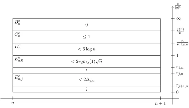
Cn={µ([n, n+ 1]×U(n/(Klogn), f(n)/K))≥2}, Dn={µ([n, n+ 1]×U(1, n/(Klogn)))≥6 logn}, En,0=µ [n, n+ 1]×U(1/√
n,1)≥2vdmλ(1)√ n ,
En,j ={µ([n, n+ 1]×U(rj+1,n, rj,n))≥2∆j,n}, n, j≥1,
(3.13)
where the numbersrj,n and ∆j,n are defined as r1,n= 1
√n, rj+1,n = sup{r >0 : ψ(r)≥ψ(rj,n) + 16 log(jf(n))},
∆j,n=ψ(rj+1,n)−ψ(rj,n) = 16 log(jf(n)), n, j ≥1.
(3.14)