Existence results for a class of p–q Laplacian semipositone boundary value problems

Existence results for a class of p–q Laplacian semipositone boundary value problems

Dedicated to Professor Jeffrey R. L. Webb on the occasion of his 75th birthday

Ujjal Das

, Amila Muthunayake

and Ratnasingham Shivaji

1The Institute of Mathematical Sciences, HBNI, Chennai, 600113, India

2Department of Mathematics and Statistics, University of North Carolina at Greensboro, Greensboro, NC 27412, USA

Received 18 June 2020, appeared 21 December 2020

Abstract. Let Ω be a bounded domain in R^N; N > 1 with a smooth boundary or Ω= (0, 1). We study positive solutions to the boundary value problem of the form:

−∆pu−∆qu=λf(u) inΩ, u=0 on∂Ω,

where q ∈ [2,p),λ is a positive parameter, and f : [0,∞) 7→ Ris a class of C¹, non- decreasing and p-sublinear functions at infinity (i.e. limt→∞ f(t)

t^p−1 =0) that are negative at the origin (semipositone). We discuss the existence of positive solutions for λ 1. Further, when p = _4,q = _{2, Ω} = (_{0, 1}) _and f(s) = (s+₁)^γ−2; γ ∈ (_{0, 3})_{, we} provide the exact bifurcation diagram for positive solutions. In particular, we observe two positive solutions for a finite range ofλand a unique positive solution forλ1.

Keywords: p–qLaplacian, semipositone problems, positive solutions.

2020 Mathematics Subject Classification: 35G30, 35J62, 35J92.

1 Introduction

In [3], authors discussed results which imply the existence of positive solutions forλ1 for the boundary value problem:

−_∆pu=λf(u) inΩ,

u=0 on ∂Ω, (1.1)

where p >_{1, Ω}is a bounded domain inR^N; N >1 with a smooth boundary, λis a positive parameter, and∆su=div|∇u|^s−2∇u);s >1, and f :[0,∞)→_Rsatisfies:

(_H1) f isC¹, non-decreasing, p-sublinear at infinity i.e. lim_t→_∞ ^f(t) t^p−1 =_0,

BCorresponding author. Emails: ujjaldas@imsc.res.in (U. Das), akmuthun@uncg.edu (A. Muthunayake), r_shivaj@uncg.edu (R. Shivaji)

(H2) f(0)<0,

(H3) limt→_∞ f(t) =_∞.

In the literature, such problems where f(0) <0, are referred as semipositone problems. It is well known that establishing the existence of a positive solution for semipositone problems are challenging, see [1,4,9,10] and references therein.

In recent years, there has been considerable interest to study boundary value problems involving the p–qLaplacian operator (−_∆p−_∆q, q∈ (1,p)), for examples, see [2,5,8,11] and the references therein. Such operators often occur in the mathematical modelling of chemical reactions and plasma physics. In this article, we extend this study ofp–qLaplacian boundary value problem for a class of semipositone reaction terms. Namely, we study the boundary value problem

−_∆pu−_∆qu=λf(u) in Ω,

u=0 on ∂Ω, (1.2)

forq∈[2,p). We establish the following result.

Theorem 1.1. Assume(H1),(H2)hold and there exists A>0,σ>0such that f(s)≥ As^σ, for s 1.

Then(1.2)has a positive solution forλ1.

Remark 1.2. It is easy to see that (1.2) does not admit any positive solution for λ ≈ 0. This follows due to the p-sublinear condition at infinity which implies there exists a M > 0 such that f(s) ≤ Ms^p−1,∀s > 0. Hence, if u is a positive solution, multiplying (1.2) by u and integrating we obtain

Z

Ω|∇u|^pdx+

Z

Ω|∇u|^qdx≤λM Z

Ω|u|^pdx which implies

λ≥ 1

M R

Ω|∇u|^pdx R

Ω|u|^p dx

!

≥ ^λ1,p M ,

whereλ_1,p>0 is the principal eigenvalue of−_∆pon Ωwith Dirichlet boundary condition.

We will use the method of sub-super solutions to establish Theorem 1.1. We will adapt and extend the ideas used in [3] to construct a crucial positive sub-solution.

Finally, for the case when Ω= (0, 1), p= 4 andq= 2, namely to the two-point boundary value problem:

−[(u⁰)³]⁰−[(u⁰)]⁰ =λf(u) in(0, 1),

u(0) =0=u(1) ^(1.3)

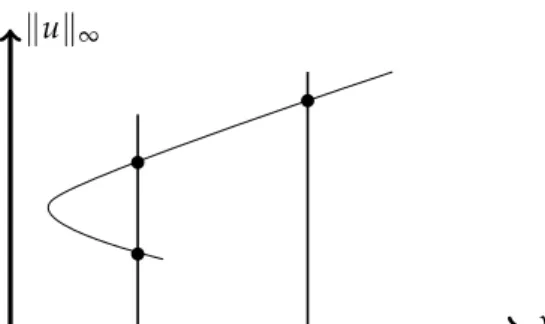
with f(s) = (s+1)^r−2; r ∈ (0, 3), we will provide exact bifurcation diagrams for positive solutions in Section 4. Bifurcation diagrams we obtained are of the form given in Figure1.1.

Note that this bifurcation diagram implies the existence of two positive solutions for certain finite range ofλand a unique positive solution forλ1.

The rest of the paper is organized as follows. In Section2, we will recall some important results that are required for the development of this article. Section3is dedicated to the proof of Theorem 1.1, and Section 4 is devoted to obtaining the bifurcation diagram of positive solutions to (1.3).

λ kuk_∞

•

•

•

Figure 1.1: Bifurcation diagram for positive solutions to (1.3)

2 Preliminaries

In this section, we recall some results concerning a sub-super solution method for p–qLapla- cian boundary value problem. First, by a weak solution of (1.2) we mean a function u ∈ W₀^1,p(_Ω)which satisfies:

Z

Ω|∇u|^p−2∇u.∇φ+

Z

Ω|∇u|^q−2∇u.∇φ=λ Z

Ωf(u)φ, ∀φ∈ C₀^∞(_Ω).

However, in this paper, we in fact study C¹(_Ω) solution. Next, by a sub-solution (super solution) of (1.2) we mean a function v ∈ W^1,p(_Ω)∩C¹(_Ω) such that v ≤ (≥)0 on ∂Ω and satisfies:

Z

Ω|∇v|^p−2∇v.∇φ+

Z

Ω|∇v|^q−2∇v.∇φ≤(≥)λ Z

Ω f(v)φ, ∀φ∈C₀^∞(_Ω), φ≥0 inΩ.

Then the following sub-super solution result holds.

Lemma 2.1. Letψ, z be sub and super solutions of (1.2)respectively such thatψ≤z inΩ.Then(1.2) has a solution u∈C¹(_Ω)such thatψ≤ u≤z.

Proof. We refer to Corollary 1 of [6] for the proof.

3 Proof of Theorem 1.1

In this section, we use sub-super solution method to prove Theorem1.1. We adapt and extend the ideas used in [3] to construct a crucial positive sub-solution.

Construction of a sub-solution: Let λ₁ be the principal eigenvalue and φ₁ ∈ C^∞(_Ω)be the corresponding eigenfunction of

−_∆φ1 =λ₁φ₁ inΩ, φ₁ =0 on∂Ω

such thatφ₁ >0 inΩandkφ₁k_∞ =1. Then∆pφ₁,∆qφ₁are inL^∞(_Ω), since 2≤q< p. Further, by Hopf’s lemma|∇φ₁|>_{0 on}∂Ω. Now we consider

ψ=λ^rφ₁^β, where β= ^p

p−1 andr ∈ 1

p−1, 1 p−1−σ

.

Note that without loss of generality we can assumeσ<q−1. Then, fors= p,q,

−_∆sψ=λ^r(s−1)β^s−1φ₁^{(β−1)(s−1)}[−_∆sφ₁]−λ^r(s−1)β^s−1(β−1)(s−1) |∇φ₁|^s φ₁^{s−β(s−1)}

.

Note thats−β(s−1) = 0 whens = pands−β(s−1) >0 whens = q. Also,|∇φ₁| >0 on

∂Ω,φ₁=0 on ∂Ωandφ₁∈ C^∞(_Ω). Therefore, by continuity, there exists aδneighborhood of

∂Ω, sayΩδ = {x∈_Ω:dist(x,∂Ω)≤δ}_{such that}

−_∆sψ<0 in Ωδ (3.1)

fors = p,q. Further, since∆pφ₁∈ L^∞(_Ω)we see that∃ e_p >0 (independent ofλ) such that

−_∆pψ≤ −λ^r(p−1)e_p inΩδ. Asr(p−₁)>_{1, for}λ1 it follows that

−_∆pψ≤ −λ^r(p−1)e_p ≤λf(0)≤λf(ψ) inΩδ. Hence, by (3.1) forλ1 we have

−_∆pψ−_∆qψ≤ λf(ψ) inΩδ. (3.2) Next let µ > 0 be such that φ₁^β ≥ µ in Ω\_Ωδ and Ms > 0 (s = p,q) be such that −_∆sψ ≤ M_sλ^r(s−1) inΩ. Sincer < _s−1¹₋

σ (s= p,q), it follows that forλ1 we have

−_∆sψ≤ M_sλ^r(s−1)≤ λA

2

(λ^rµ)^σ

≤ λ

2

f(ψ) _inΩ\_Ωδ. Thus, forλ1, we obtain

−_∆pψ−_∆qψ≤λf(ψ) inΩ\_Ωδ. (3.3) Combining (3.2) and (3.3), forλ1 we see that

−_∆pψ−_∆qψ≤λf(ψ) in Ω. (3.4)

Therefore,ψis a sub-solution of (1.2) whenλ1.

Construction of a super solution:LetR>0 be such thatΩ⊆B_R(0), whereB_R(0)is the open ball of radiusRcentered at origin. Now consider

η(r) = ¹−(_R^r)^p0

p⁰ onB_R, where ¹_p + _p¹₀ =1. Notice that 0≤η≤1. Also for 0≤r≤ R,

η⁰(r) =−^r

p⁰−1

R^p0 ,

−_∆sη=− |η⁰(r)|^s−2η⁰(r)⁰ = ^r

(p⁰−1)(s−1)

R^p0(s−1)

!0

≥0 in B_R, (3.5)

fors= p,q. In particular,

−_∆pη= ¹

R^p. (3.6)

Now let Z = M(λ)η, where M(λ) 1 so that ^[M_f(⁽_M^λ)]₍^p−1

λ)) ≥ λR^p. Note that this is possible by (H1). Then, using that f is non-decreasing, (3.5) and (3.6) we have

−_∆pZ−_∆qZ≥ −_∆pZ= ^M(λ)^p−1

R^p ≥λf(M(λ))≥λf(Z)inBR. (3.7) ClearlyZ≥0 on ∂Ωand hence it is a super solution of (1.2).

Proof of Theorem1.1. Let ψ be a sub-solution of (1.2) for λ 1 (as constructed in (3.4)).

Then, we can construct a super solution Z of (1.2) (as constructed in (3.7)). Further, since Z>0 inΩ, we can choose M(λ)1 such thatZ≥ ψin Ω. Hence by Lemma2.1, (1.2) has a positive solutionu_λ ∈ [ψ,Z]forλ1 and Theorem1.1is proven.

4 Bifurcation diagram for positive solutions to (1.3)

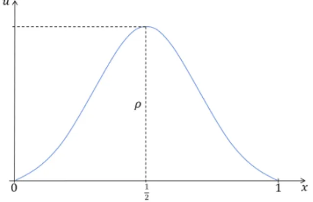
Here we adapt and extend the method used by Laetsch in [7] where he studied the boundary value problem: −u⁰⁰ = λf(u);(0, 1), u(0) = 0 = u(1). First we note that since (1.3) is au- tonomous, any positive solution umust be symmetric about x = ¹₂, increasing on(0,¹₂), and decreasing on(¹₂, 1). Letu(¹₂) =ρ(say).

Figure 4.1: Shape of a positive solution to (1.3) Now multiplying (1.3) byu⁰ and integrating we obtain

−³

4[(u⁰)⁴]⁰−¹

2[(u⁰)²]⁰ = λ(F(u))⁰ in(0, 1) where F(s) =Rs

0 f(z)dz. Further integrating we obtain

3[u⁰(x)]⁴+2[u⁰(x)]² =4λ[F(ρ)−F(u(x))] in [0,¹₂] and hence

u⁰(x) = r

1+12λ(F(ρ)−F(u(x)))

1 2−1

√3 in [0,¹₂]. (4.1)

Figure 4.2: Shape of a function F

Noting thatu⁰(0) =

q

[1+12λF(ρ)]¹2−1

√3 , it is easy to see thatρmust be greater or equal toθ where θ is the position zero ofF. Integrating (4.1) we get

Z _u(x) 0

ds q

1+12λ(F(ρ)−F(s))¹² −1

= √^x

3 in [0,¹₂), (4.2) and settingx→(¹₂)⁻we obtain

G(_λ,ρ) =

Z _ρ

0

ds q

1+12λ(F(ρ)−F(s))¹² −1

= ¹ 2√

3. (4.3)

Figure 4.3: Bifurcation diagrams for (1.3) when f(s) = (s+1)^γ −2; γ = 0.85, 1.25, 1.5, 2.0, 2.5.

It can be shown that that for λ > 0 and ρ ≥ θ, G(λ,ρ)is well defined. Further, if λ > 0, ρ ≥ θ satisfies (4.3), then (4.2) yields aC² function u : [0,¹₂) → [0,ρ) such thatu(x) → ρ as x→(¹₂)⁻. Extending this function on[0, 1]so thatu(¹₂) =ρ, and it is symmetric aboutx= ¹₂, it can be shown that it will be a positive solution of (1.3). Hence the bifurcation diagram for positive solutions to (1.3) is given by:

S= (λ,ρ)|λ>0,ρ≥θ &G(λ,ρ) = ¹

2√

3 . (4.4)

Now, when f(s) = (s+1)^γ −2; γ ∈ (0, 3), we compute S using Mathematica. In partic- ular, here are the bifurcation diagrams we obtained for γ = 0.85, 1.25, 1.5, 2.0 and 2.5 (see Figure4.3).

References

[1] H. Berestycki, L. A. Caffarelli, L. Nirenberg, Inequalities for second order elliptic equations with applications to unbounded domains, I. A celebration of John F. Nash Jr., Duke Math. J. 81(1996), No. 2, 467–494. https://doi.org/10.1215/S0012-7094-96- 08117-X;MR1395408;Zbl 0860.35004.

[2] V. Bobkov, M. Tanaka, On positive solutions for (p,q)-Laplace equations with two parameters, Calc. Var. Partial Differential Equations 54(2015), No. 3, 3277–3301. https:

//doi.org/10.1007/s00526-015-0903-5;MR3412411.

[3] D. D. Hai, R. Shivaji, An existence result on positive solutions for a class of p-Laplacian system, J. Math. Anal. Apl. 56(2004), No. 7, 1007–1010. https://doi.org/10.1016/j.

jmaa.2007.01.067;MR2038734.

[4] A. Castro, M. Chhetri, R. Shivaji, Nonlinear eigenvalue problems with semipositone structure, in: Proceedings of the Conference on Nonlinear Differential Equations (Coral Gables, FL, 1999), Electron. J. Differ. Equ. Conf. Vol. 56, Southwest Texas State Univ., San Marcos, TX, 2000, pp. 33–49.MR1799043;Zbl 0959.35045.

[5] L. Cherfils, Y. Il’yasov, On the stationary solutions of generalized reaction diffusion equations with p&q-Laplacian, Commun. Pure Appl. Anal. 4(2005), No. 1, 9–22. https:

//doi.org/10.3934/cpaa.2005.4.9;MR2126276;Zbl 1210.35090.

[6] L. F. O. Faria, O. H. Miyagaki, D. Motreanu, M. Tanaka, Existence results for nonlinear elliptic equations with Leray–Lions operator and dependence on the gradient, Nonlin- ear Anal. 96(2014), 154–166. https://doi.org/10.1016/j.na.2013.11.006; MR3143809;

Zbl 1285.35014.

[7] T. Laetsch, The number of solutions of a nonlinear two point boundary value problem, Indiana Univ. Math. J.20(1970), No. 1, 1–13.MR0269922.

[8] G. Li, X. Liang, The existence of nontrivial solutions to nonlinear elliptic equation of p–q-Laplacian type on R^N, Nonlinear Anal. 71(2009), No. 5–6, 2316–2334.https://doi.

org/10.1016/j.na.2009.01.066;MR2524439;Zbl 1171.35375.

[9] P. Lions, On the existence of positive solutions of semilinear elliptic equations,SIAM Rev.

24(1982), No. 4, 441–467.MR0678562.

[10] S. Oruganti, J. Shi, R. Shivaji, Diffusive logistic equation with constant yield harvesting, I. Steady states, Trans. Amer. Math. Soc. 354(2002), No. 9, 3601–3619.https://doi.org/

10.1090/S0002-9947-02-03005-2;MR1911513;Zbl 1109.35049.

[11] H. R. Quoirin, An indefinite type equation involving two p-Laplacians, J. Math.

Anal. Appl. 387(2012), No. 1, 189–200. https://doi.org/10.1016/j.jmaa.2011.08.074;

MR2845744;Zbl 1229.35074.