arXiv:1804.01837v1 [math.DS] 5 Apr 2018
ZOLT ´AN BUCZOLICH* AND GABRIELLA KESZTHELYI**
Abstract. We consider skew tent mapsTα,β(x) such that (α, β)∈[0,1]2is the turning point ofTα,β, that is,Tα,β= βαxfor 0≤x≤αandTα,β(x) = 1−βα(1−x) forα < x ≤1. We denote by M =K(α, β) the kneading sequence ofTα,β, by h(α, β) its topological entropy and Λ = Λα,β denotes its Lyapunov exponent.
For a given kneading squence M we consider isentropes (or equi-topological entropy, or equi-kneading curves), (α,ΨM(α)) such that K(α,ΨM(α)) = M. On these curves the topological entropyh(α,ΨM(α)) is constant.
We show that Ψ′M(α) exists and the Lyapunov exponent Λα,β can be expressed by using the slope of the tangent to the isentrope. Since this latter can be computed by considering partial derivatives of an auxiliary function ΘM, a series depending on the kneading sequence which converges at an exponential rate, this provides an efficient new method of finding the value of the Lyapunov exponent of these maps.
1. Introduction
Consider a point (α, β) in the unit square [0,1]2. Denote by Tα,β(x) the skew tent map.
(1) Tα,β(x) =
Lα,β(x) = αβx if 0≤x≤α, Rα,β(x) = 1−αβ (1−x) if α < x≤1.
To avoid trivial dynamics we suppose that 0.5 < β ≤ 1 and α ∈ (1− β, β).
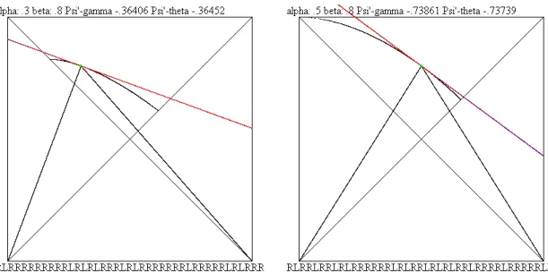
We denote by U the region of [0,1]2 consisting of these [α, β]. We denote by M = K(α, β) the kneading sequence of Tα,β, by h(α, β) its topological entropy and by Λ = Λα,β denotes its Lyapunov exponent. The set of all possible kneading sequences is denoted byM={K(α, β) : (α, β)∈U}.For a given kneading squence M we consider isentropes (or equi-topological entropy, or equi-kneading curves) (α,ΨM(α)) ∈ U such that K(α,ΨM(α)) = M. On these curves the topological entropy h(α,ΨM(α)) is constant. On Figure 1 on the left half T.3,.8 is considered.
The first listed author was supported by the Hungarian National Foundation for Scientific Re- search Grant 124003. During the preparation of this paper this author was a visiting researcher at the R´enyi Institute.
The second listed author was supported by the Hungarian National Foundation for Scientific Research Grant 124749.
2000 Mathematics Subject Classification: Primary 37B25; Secondary 28D20, 37B40, 37E05.
Keywords: skew tent map, topological entropy, isentrope, invariant measure, Lyapunov expo- nent, Markov partition.
1
On the bottom part of the figure one can see the first few entries of the kneading sequence. To visualize the isentrope the computer plotted in black some pixels which correspond to parameter values with similar initial segment of kneading sequence. To obtain a not too thick region the length of this initial segment depends on the parameter region. For example on the left half of Figure 2 there is a thicker region, which can be made thinner by considering longer initial segments.
However if the initial segment is too long, the computer is not finding enough pixels from the given equi-kneading region, see for example the right half of Figure 1 where close to the upper left corner of the unit square the plot is too thin.
Figure 1. Tangents to isentropes computed from γ and from Θ
We will see in this paper that the isentropes (α,ΨM(α)) are continuously dif- ferentiable curves. What we found really interesting that the derivatives of these curves can be used to compute the Lyapunov exponents of the skew tent maps Tα,β.
To study equi-topological entropy, or equi-kneading curves in the region U in [4] we introduced the auxiliary functions ΘM. Suppose that we have a given kneading-sequence M and
(2) M− =R L . . . L| {z }
m1
R L . . . L| {z }
m2
R L . . . L| {z }
m3
R . . . .
HereM =M− if the turning point is not periodic, that is Tα,βk (α)6=α for k ∈N. In this case there is no C ∈M. The set of such kneading sequences is denoted by M∞. The cases when the truning point is periodic, that is when C appears in M will play a very important role in this paper. The set of these kneading sequences is denoted by M<∞. These are the ones ending with C. In this case M− can be defined in many ways. One such way was discussed in [4]. However, for our
α β γ Ψ′M–γ Ψ′M–Θ .3 .8 .20444 -.36406 -.36452 .49 .56 .30996 -.40344 -.4244 .5 .7 .27034 -.64303 -.64064 .5 .8 .26918 -.73861 -.73739 .6 .75 .35597 -.76258 -.76132 .6 .9 .47736 -.4599 -.45991 Table 1. Tangents calculated from Θ and γ
definition of suitable ΘM functions any of the following definitions can be used.
Concatenate M with itself infinitely many times. Then in the right infinite (right) periodic sequence replace the Cs in an arbitrary manner withRs and Ls.
For example in our computer simulations each C was replaced by an L. This is due to the fact that if Tα,βk (α) = α then Tα,βk+1(α) = β = Lα,β(Tα,βk (α)) = Rα,β(Tα,βk (α)), that is both the left- and right- “half definitions” of Tα,βk can be used in this case.
We put mk=m1 +m2+· · ·+mk with mi defined in (2) and (3) ΘM(α, β) = 1−β+
X∞
k=1
(−1)k
1−α β
k α β
mk
.
In [4] we showed that for (α, β)∈U it follows fromK(α, β) =M that ΘM(α, β) = 0. This means that the equi-topological entropy curve{(α, β)∈U :K(α, β) =M} is a subset of {(α, β)∈ U : ΘM(α, β) = 0}, the zero level set of ΘM. This means that the isnetrope (α,ΨM(α)) satisfies the implicit equation ΘM(α,ΨM(α)) = 0.
By implicit differentiation
(4) Ψ′M(α) = −∂1ΘM(α,ΨM(α))
∂2ΘM(α,ΨM(α)),
provided that ∂2ΘM(α,ΨM(α))6= 0. Since the series in (3) converges at an expo- nential rate if we consider the partial derivatives we also obtain an exponential convergence rate for the partial derivatives and hence it is very easy to com- pute/approximate Ψ′M(α) by using (4). On Figures 1, 2 and in Table 1 the entries Psi’-theta and Ψ′M − Θ were computed by using this implicit differentiation method by taking into consideration the first 200 elements of the kneading se- quence.
The other approach is to estimate Ψ′M(α) via the Lyapunov exponents. For the skew tent map Tα,β, (α, β) ∈ U there is a unique ergodic acim µα,β = µ, that is a measure absolutely continuous with respect to the Lebesgue measure, λ. Its density f is an invariant function/fixed point of the Frobenius-Perron operator
Pα,β, that is Pα,βf =f. By Birkhoff’s ergodic theorem the Lyapunov exponent (5) Λα,β = lim
N→∞
1
N log|(Tα,βN )′(x)|= lim
N→∞
1 N
N−1X
n=0
log|Tα,β′ (Tα,βn (x))| for µ. a.e. x.
In case of skew tent maps |Tα,β′ (x)| = β/α if x < α and |Tα,β′ (x)| = β/(1−α) if x > α hence if we let
(6) γ = lim
N→∞
1 N
N−1X
n=0
χ[0,α](Tα,βn (x)) then Λα,β =γlogβ
α + (1−γ) log β 1−α, for µa.e. x.
Figure 2. More tangents to isentropes computed from γ and from Θ Hence to estimate the Lyapunov exponent we need to estimateγ. This is usually done by using a computer program. For a sufficiently large N and a “randomly”
selected xone computes the sum in (6). Actually we have done this as well in our computer simulations. It has turned out thatN = 200000 was sufficiently large to have a reasonably good estimate for γ. In Table 1 there is a columnγ containing these estimates for the randomly selected parameter values. The main result of this paper is the fact that γ, and hence Λα,β can be expressed by using Ψ′M(α).
We show in Proposition 10 and in Theorem 13 that (7) γ =α(1−α)Ψ′M(α)
β +α or, taking inverese Ψ′M(α) = (γ−α)β α(1−α).
Since Ψ′M(α) can be calculated by (4) using (5), (6) and (7) we can calculate the Lyapunov exponent for any Tα,β with (α, β)∈U.To illustrate the connection between Ψ′M(α) and Λα,β, or γ in our computer simulations followed a reverse
approach. This means that the computer program calculated an estimate ofγ(and hence of Λ) and this estimate was used for calculating the slope of an approximate tangent to the isentrope. As the images show this method, based on (7) works, that is the approximate tangents really seem to be tangent to the isentrope.
In Table 1 there is a column labeled Ψ′M–Θ which contains the estimates we obtained for Ψ′M(α) by using the estimate for γ based on (6). As one can see that the estimates we obtained for Ψ′M(α) by using the ΘM function in (4) are quite close to the ones obtained by using γ. On Figures 1 and 2 we plotted both approximate tangents to the isentropes, the one calculated from γ and the one calculated from ΘM. On the color pdf version of the paper the first approximate tangent is in red and the second is in blue. In case only one, the red tangent is visible then it means that the two approximate tangents are on top of each other. It is also visible that they are indeed ”tangent” to the isentrope as well. On the right half of Figure 2 the two approximate tangents are not exactly on top of each other. This is due to the fact that for the parameter values α = 0.49 and β = 0.56 both α/β and (1−α)/β are close to one and the convergence in the series giving the partial derivatives of ΘM is slower. To get a better estimate one needs to consider more than the first 200 entries of the kneading sequence. On this figure the tiny black region corresponding to the equi-kneading region is almost completely covered by the blue and red approximate tangents. We would like to emphasize that our new method based on ΘM, even if the number of iterates is increased from 200 to a larger number requires still much less many iterates than the other method which needed 1000 times more iterates for about the same accuracy.
Finally, there is one more illustration showing that indeed there is a link between γ and Ψ′M(α). On Figure 3 the color of pixels in U was calculated based on the first 10 entries of the kneading sequence. Hence equi-kneading regions containing isentropes are of the same color (modulo screen/pixel resolution). We also plotted three skew tent maps with three different colors and the approximate tangent line computed by using γ from (6) substituted into (7).
As far as we know in the literature there were two ways to estimate/approximate Lyapunov exponents of skew tent maps. One method is based on computer pro- grams approximating γ, or the acim, or its density as we also did in some calcula- tions on our illustrations. In [2] for the Markov case a histogram of the distribution of the location in the Markov partition of the first 50000 iterates of a ”generic”
point is used to approximate the piecewise constant invariant density function of the acim. Here again a rather high number of iterates was used. In [7] a central limit theorem is discussed for the convergence in (6). The other method, discussed in [2] is based on the fact that if K(α, β)∈M<∞, that is when the turning point is periodic for Tα,β then there is a Markov partition forTα,β. Based on the Markov partition one can obtain a system of linear equations and the solution of this sys- tem gives us the invariant density function fα,β of the acim µα,β of Tα,β. Then γ =µα,β([0, α]). (In [2] a different parametrization and notation was used, but we
translated it to our notation.) The drawback of this calculation is that the number of equations is the number of elements in the Markov partition. If K(α, β)∈M∞ then there is no Markov partition, but isentropes corresponding to skew tent maps with Markov partition are dense in U. It was remarked in [2] that in this case we can also approximate the invariant density by invariant densities of Markov skew tent maps. In this case the number of elements in the Markov partition of these appproximating maps tends to infinity, making it more and more difficult to solve the system of linear equations. It also seems for us that Theorem 10.3.2 from [3] was used in an incorrect way in [2]. By this we mean, that the way these Markov skew tent maps are approximating the non-Markov one is not satisfying the exact assumptions of Theorem 10.3.2 in [3]. Since in our paper we also need approximations of skew tent maps by other ones in Proposition 6 we clarify the way these approximations work. For some specific Markov parameter values in [10] a central limit behavior is discussed.
Properties of isentropes, especially connectedness in different families of dynam- ical systems were also studied for example in [1], [9] and [12].
Figure 3. Isentropes and tangents computed from γ
This paper is organized the following way. In Section 2 we recall some defini- tions and results concerning skew tent maps and invariant densities. In Section 3
we continue to discuss some known results about absolutely continuous invariant measures and prove Proposition 6 which will be the key lemma about approxima- tions of skew tent maps by other ones. This section concludes with some remarks about uniform Lipschitz properties of isentropes.
The most involved part of the paper is Section 4 in which we prove Proposition 10. This is a special version of the main result of the paper about the relationship between Lyapunov exponents and tangents to isentropes. In this proposition we suppose that the isentrope is differentiable at the point considered and we also suppose that we work with a Markov map. In later sections we aim towards Theorem 13 to use some approximation arguments to remove the assumptions about differentiability and Markovness.
In Section 5 by using Proposition 10 first we show that isentropes are continu- ously differentiable for Markov skew-tent maps. In this argument we use Propo- sition 6 and approximations of our skew tent map by other ones with the same topological entropy. Then by using another approximation argument based on Proposition 6 and approximation of non-Markov maps by Markov maps we gener- alize this result for arbitrary maps.
Finally, in Section 6 we prove Theorem 13 which is the main result of our paper.
It is again an approximation argument of non-Markov maps by Markov maps.
This way we obtain the general version of Proposition 10.
2. Preliminaries
Kneading theory was introduced by J. Milnor and W. Thurston in [8]. For symbolic itineraries and for the kneading sequences we follow the notation of [6].
Suppose T = Tα,β is fixed for an (α, β) ∈ U and x ∈ [0,1]. The extended kneading sequence K(α, β) = Mext = (m1,m2, ...) ∈ {L, R, C}N is defined as follows. IfTα,βn (α)< αthenmn =L, if Tα,βn (α) = αthenmn=C, and ifTα,βn (α)>
α then mn =R. If there is no C in Mext then the kneading sequence K(α, β) = M =Mext. If there are Cs in Mext then the kneading squence K(α, β) =M is a finite string which is obtained by stopping at the first C and throwing away the rest of the infinite string Mext.
Following notation of [11] we denote by M the class of kneading sequences K(0.5, β), β ∈(0.5,1], which is identical to all possible kneading sequences of the form K(α, β), (α, β)∈U.
In [11] a different parametrization of skew tent maps was used. The functions Fλ,µ(x) =
1 +λx if x≤0 1−µx if x≥0 were considered on R.
A simple calculation shows that if (α, β)∈U then (λ(α, β), µ(α, β)) = (βα,1−αβ ) belongs to the region D′ = {(λ, µ) : λ > 1, µ > 1,λ1 + 1µ ≥ 1} this, apart from a boundary segment, coincides with the parameter region D = {(λ, µ) : λ ≥
1, µ > 1,1λ + µ1 ≥ 1} considered in [11]. In [4] we gave the explicit formula for the linear homeomorphism showing that Tα,β and Fλ(α,β),µ(α,β) are topologically conjugate. We use the notationK(λ, µ) for the kneading sequence ofFλ,µ. In this parametrization M corresponds to the kneading sequences of functions Fµ,µ with 1< µ ≤2.
We denote by≺the parity lexicographical ordering of kneading sequences, sym- bolic itineraries, for the details see [6].
Without discussing too much details of renormalization we need to say a few words about it. The interested reader is refered to more details in [6] or [11]. For j = 0,1, ... we denote by Mj the set of those kneading sequences M for which there exists β ∈ ((√
2)j+1,√
2j] such that M = K(12, β). The kneading sequences in M0 correspond to the non-renormalizable case. We denoute by Uj the set of those (α, β) ∈ U for which K(α, β) ∈ Mj. In [11], D0 denotes the region of those (λ, µ) ∈ D for which λ > µ2µ−1. This is the non-renormalizable region in the λ−µ-parametrization. In [2] and [11] mainly the non-renormalizable region is considered. In Section 5 of [11] renormalization, and the way of extension the result obtained for the non-renormalizable case is discussed. It turns out that if K(λ, µ) ∈ Mj with j ≥ 1 then Fλ,µ2 can be restricted onto a suitable interval mapped into itself by this map. This restriction is topologically conjugate toFµ2,λµ
and K(µ2, λµ)∈ Mj−1. In our parametrization if K(α, β) ∈ Mj with j ≥ 1 then Tα,β2 restricted onto a suitable interval is topologically conjugate to T1−α,β2/(1−α)
and K(1−α, β2/(1−α)) ∈ Mj−1. In this paper we only use that the density of Markov maps in U1, shown in [2] implies via renormalization density of Markov maps in U.
We recall a corollary of Theorem C of [11] adapted to ourα−β-parametrization.
Theorem 1. For each M ∈ M there exist two numbers α1(M) < α2(M) and a continuous function ΨM : (α1(M), α2(M))→U such that for (α, β)∈U we have K(α, β) =M if and only ifβ = ΨM(α). The graphs of the functionsΨM fill up the whole set U. Moreover, limα→α1(M)+ΨM(α) = 1 if M RLR∞. If M ≺ RLR∞ then the curve (α,ΨM(α)) converges to a point on the line segment {(α,1−α) : 0 < α < 12} as α → α1(M)+. If M = RL∞ then α1(M) = 0, α2(M) = 1 and ΨM(α) = 1 for all α ∈(0,1).
For the skew tent mapTα,β, (α, β)∈U we define the Frobenius-Perron operator Pα,β :L1[0,1]→L1[0,1] by
Pα,βf(x) = X
z∈{Tα,β−1(x)}
f(z)
|Tα,β′ (z)|, which in a more explicit form is
(8) Pα,βf(x) = α βf
αx β
+ 1−α β f
1− 1−α β x
if 0≤x≤β,
and Pα,βf(x) = 0 if x > β.
We recall for example from Proposition 4.2.4 of [3] the contraction property of Frobenius-Perron operator
(9) kPα,βfk1 ≤ kfk1.
We also remind to the definition of the variation of a real function f : [a, b]→R. V f =V[a,b]f = sup
P
( n X
k=1
|f(xk)−f(xk−1)| )
where sup is taken for all partitions P = {[x0, x1],[x1, x2], . . .[xn−1, xn]} of [a, b].
If V[a,b]f < +∞ then f is of bounded variation, BV on [a, b].
Definition 2. Suppose I = [a, b], T :I →I. A partition P ={[a0, a1],[a1, a2], . . . ,[an−1, an]}
of [a, b] is Markov for T if for any i = 1, . . . , n the transformation T|(ai−1,ai) is a homeomorphism onto the interior of the connected union of some elements of P, that is onto an interval (aj(i), ak(i)).
Observe that ifTα,βn (β) = α, that is C appears inK(α, β)∈M<∞then the parti- tion determined by the points{0, α, β, Tα,β(β), . . . , Tα,βn−1(β),1}provides a Markov partition.
3. Absolutely continuous invariant measures and densities for skew tent maps
We recall some definitions and results from [3] p. 96. We denote by T(I) the set of those transformations T :I →I which satisfy the next two properties:
I. T is piecewise expanding, that is there exists a partition P = {Ii = [ai−1, ai], i = 1, . . . , n} of I such that T|Ii is C1 and |T′(x)| ≥ α > 1 for any i and for allx∈(ai−1, ai).
II. g(x) = |T′1(x)| is a function of bounded variation, where T′(x) is an appro- priately calculated one-sided derivative at the endpoints of P.
For every n≥1 we define P(n) as P(n)=
n−1_
k=0
T−k(P) ={Ii0∩T−1(Ii1)∩· · ·∩T−n+1(Iin−1) :Iij ∈ P, j = 0, . . . , n−1}. One can easily see that if T ∈ T(I) then Tn is piecewise expanding on P(n).
Since |Tα,β′ (x)| = αβ on [0, α] and |Tα,β′ (x)| = 1−αβ on [α,1], for (α, β) ∈ U we obtain that Tα,β ∈ T([0,1]) with P ={[0, α],[α,1]}.
The next theorem is about the existence of absolutely continuous invariant mea- sures, acims and it is Theorem 5.2.1. from [3].
Theorem 3. If T ∈ T(I) then it admits an absolutely continuous invariant mea- sure, acim whose density is of bounded variation.
In case of skew tent maps this acim is unique. Theorem 8.2.1 of [3] gives an upper bound on the number of distinct ergodic acims for aT ∈ T(I).
Theorem 4. Let T ∈ T(I) be defined on a partition P. Then the number of distinct ergodic acims for T is at most #P −1.
In our case when (α, β) ∈ U and I0 = [0,1] then P = {[0, α],[α,1]}. Since
#P = 2 we obtain that for Tα,β there is only one ergodic acim. Using this and the results about the spectral decomposition of the Frobenius-Perron operator in Chapter 7 of [3] one can see that invariant densities are linear combinations of densities of ergodic acims. Hence in case of our skew tent maps the following Lemma holds:
Lemma 5. For every (α, β)∈U there is a unique invariant density for Tα,β, and it is the density of the unique ergodic acim.
As Theorems 10.2.1 and 10.3.2 are proved in [3] we show the next proposition.
Proposition 6. Suppose (αn, βn)∈U for n = 0,1, . . . , (αn, βn)→(α0, β0) and Pn ={[0, αn],[αn,1]}. Suppose that
∀m≥1,∃δm >0 such that if Pn(m) =
m−1_
j=0
Tα−jn,βn(Pn) then min
I∈Pn(m)
λ(I)≥δm >0.
(10) Then:
(A) For any density f of bounded variation there exists a constant M such that for any n and k = 1,2, . . .
V Pαkn,βnf ≤M.
This implies that for any n there is an invariant density fn of Tαn,βn and the set {fn} is a precompact set in L1([0,1], λ).
(B) Moreover, if fnk →f0 in L1 then f0 is an invariant density for Tα0,β0.
In a similar situation in [2] there is a direct reference to Theorem 10.3.2 of [3] but it seems that after a careful check, this reference is not applicable in the situation of the Markov approximations in [2], neither in our case.
Next we discuss what the problem is with the direct application of Theorem 10.3.2 then by using the ideas of the proofs of Theorems 10.2.1 and 10.3.1 of [3]
we prove our Proposition 6.
The main problem of the direct application in [2] of the theorems from [3] to the case of approximations by skew tent maps is the following. In the assumptions of these theorems given a piecewise expanding transformation T : I → I, a family {Tn}n≥1of approximating Markov transformations associated withT is considered.
Assume Q(0) denotes the endpoints of intervals belonging to P(0), where P(0) is a partition such that T is C1 and expanding on the partition intervals of P(0).
If one checks in Section 10.3, p. 217 of [3] the definition of the approximating Markov transformations associated with T one can see that there is a sequence of partitionsP(n). It is supposed that the transformationsTnare piecewise expanding and Markov transformations with respect to P(n).
Moreover, in assumption (a) on p. 217 of [3] it is stated that if J = [c, d]∈ Pn and J ∩ Q(0) =∅ then Tn|J is a C1 monotonic function such that
(11) Tn(c) = T(c), Tn(d) =T(d)
Assumption (11) is clearly not satisfied if (αn, βn)→(α0, β0), (αn, βn)6= (α0, β0), Tn =Tαn,βn,T =Tα0,β0 and P(n) has subintervals [c, d] which do not contain 0, α0
or 1. This means that contrary to what is claimed by the authors of [2] Theorem 10.3.2 of [3], cannot be applied directly to the case of Markov approximations they want to use. Our Proposition 6 can be used in their case as well. Moreover, it is also an advantage of our Proposition 6 that we do not assume that the approximating skew tent maps are Markov.
Proof of Proposition 6. First we check that assumptions of Theorem 10.2.1 in [3]
are satisfied by Tαn,βn and Tα0,β0 given in Proposition 6. First observe that by (αn, βn)→(α0, β0) we can chooseγ >1 such that|Tα′n,βn(x)| ≥γfor anyxwhere the derivative exists for any n, this implies condition (1) of Theorem 10.2.1 of [3].
Since |T′1
αn,βn| is constant on (0, αn) and (αn,1), from (αn, βn)→(α0, β0) it clearly follows that there exists W > 0 such that V
1 Tαn,βn′
≤ W for any n ∈ N. This shows that condition (2) of Theorem 10.2.1 of [3] is also satisfied. Observe that by (αn, βn) → (α0, β0) the partitions Pn have the property that we can choose δ > 0 such that ifI ∈ Pn then Tαn,βn|I is one-to-one, Tαn,βn(I) is an interval and minI∈Pnλ(I)> δ. This is condition (3) of Theorem 10.2.1 of [3].
Finally, (10) is assumption (4) of Theorem 10.2.1. Therefore this theorem is applicable to the sequence Tαn,βn. This yields that conclusion (A) of our Proposi- tion 6 holds true. The only thing which needs extra proof that in conclusion (B) the function f0, which is the L1 limit of the P0αnk,βnk invariant densities fnk, is Pα0,β0 invariant. Since fnk → f0 in L1 and R
fnk = 1 for all k, it is clear that
|R
f0−R
fnk| ≤R
|f0−fnk| →0 and henceR
f0 = 1.
For the invariance off0 we need to show thatPα0,β0f =f0 a.e.. As on page 220 of [3] it is sufficient to show that kPα0,β0f0 −f0k1 = 0, which will be verified by the following estimates:
kPα0,β0f0−f0k1 ≤ kPα0,β0f0−Pαnk,βnkf0k1+kPαnk,βnkf0 −Pαnk,βnkfnkk1 +kPαnk,βnkfnk−fnkk1+kfnk −f0k1 =A1,nk +A2,nk +A3,nk +A4,nk.
By (9), A2,nk ≤ kPαnk,βnkk1· kf0 −fnkk1≤ kf0−fnkk1 →0.
Sincefnk is an invariant density ofTαnk,βnk we have A3,nk = 0 for any k. It is also clear that A4,nk →0 ask → ∞.
The only non-trivial part is the estimation ofA1,nk. Suppose ε >0 is given and choose an fε ∈C1[0,1] such that kf0−fεk1 < ε. Put
(12) Mε = max{|fε(x)|+|fε′(x)|:x∈[0,1]}. We suppose that K0 is chosen in a way that
α0
β0 − αnk
βnk
< ε
Mε
, 1−α0
β0 − 1−αnk
βnk
< ε
Mε
, and |βk−β0|
βk
< ε Mε
hold for k ≥K0. (13)
We suppose that βnk ≥ β0, the case βnk < β0 is similar and is left to the reader.
For ease of notation we denote nk by k in the sequel. We have fork ≥K0
A1,k =kPα0,β0f0−Pαk,βkf0k1 ≤ kPα0,β0fε−Pαk,βkfεk1 +kPα0,β0k · kf −fεk +kPαk,βkk · kf0−fεk
(using (9))
≤ kPα0,β0fε−Pαk,βkfεk+ 2ε≤ Z β0
0
α0
β0
fε
α0
β0
x
− αk
βk
fε
αk
βk
xdx
+ Z β0
0
1−α0
β0
fε
1−1−α0
β0
x
− 1−αk
βk
fε
1−1−αk
βk
xdx +
Z βk
β0
αk
βk
fε αk
βk
x+ 1−αk
βk
fε
1− 1−αk βk
xdx+ 2ε
≤ Z β0
0
α0
β0
fε
α0
β0
x
−fε
αk
βk
x+ α0
β0 − αk
βk
fε
αk
βk
x
dx +
Z β0
0
1−α0 β0
fε
1− 1−α0 β0
x
−fε
1−1−αk βk
x +
1−α0
β0 − 1−αk
βk fε
1− 1−αk
βk x
dx+|βk−β0| αk
βkMε+ 1−αk
βk Mε
+ 2ε (using (12) and (13))
< α0
β0
Mε
α0
β0 −αk
βk
Z β0
0 |x|dx+β0
α0
β0 −αk
βk
·Mε
+1−α0
β0
1−α0
β0 −1−αk
βk
·Mε·
Z β0
0 |x|dx+β0
1−α0
β0 − 1−αk
βk
·Mε+ε+ 2ε
(using again (13))
< α0
β0 ·ε+β0 ·ε+1−α0
β0
ε+β0·ε+ 3ε <
1 β0
+ 2β0+ 3
ε.
Thus kPα0,β0f −Pαk,βkfk1 → 0 as k → ∞ and hence A1,k → 0 as k → ∞ and
completes the proof of the Proposition.
The next lemma shows that if Tα0,β0 is non-Markov, that is K(α0, β0) ∈ M∞ then (10) is satisfied.
Lemma 7. Suppose(α0, β0)∈U, K(α0, β0) =M ∈M∞.The sequence(αn, βn)→ (α0, β0), (αn, βn)∈U, Pn ={[0, αn],[αn,1]}, n = 0,1, . . . then (10) is satisfied.
Proof. Since M ∈M∞ we have Tαk+10,β0(α0) =Tαk0,β0(β0)6=α0 for k = 0,1, . . . . This implies that
(14) Tαk+10,β0(α0)6=Tαk0′,β0(α0) ifk′ > k ≥0.
Observe that the division points of Pn(m), (n = 0,1, . . .) are 0,1 and points of the form Tα−jn,βn(αn) with 0≤j ≤m−1. Denote the set of division points of Pn(m) by Q(m)n . By (14) we have
(15) α0 ∈/ Tα−j0,β0(α0) for any j = 1,2, . . . and in general
(16) Tα−j0,β′0(α0) and Tα−j0,β0(α0) are disjoint finite sets for j′ 6=j.
Indeed, if we had for a j′ > j ≥1, x∈Tα−j0,β′0(α0) ∩ Tα−j0,β0(α0) then Tαj0′−j,β0(Tαj0,β0(x)) =α0 =Tαj0,β0(α0)
and hence Tαj0′−j,β0(α0) =α0, which contradicts (14).
Denote byδ0,mthe length of the shortest interval inP0(m). By usingαn →α0, βn→ β0, (15) and (16) we can select Nm such that
(17) distHau(Q(m)n ,Q(m)0 )< δ0,m/3 holds for n≥Nm. This implies that for minI∈P(m)
n λ(I) ≥ δ0,m/3 > 0 holds for n ≥ Nm. Since min{λ(I) :I ∈ Pn(m), n ≤Nm}>0 we obtain that (10) is satisfied.
Finally, in this section we make a few remarks about the Lipschitz property of the isentropes. By Theorem A of [11] if µ′ > µ and λ′ > λ then the topological entropy of Fλ′,µ′ is larger than that of Fλ,µ. Recalling that λ= βα and µ= 1−αβ we obtain that if the isentrope{(α,ΨM(α)) :α∈(α1(M), α2(M))}is passing through the point (α0, β0) = (α0,ΨM(α0)) then
(18) ΨM(α)−ΨM(α0)
α−α0 ≤ β0
α0 for α > α0
and
(19) ΨM(α)−ΨM(α0)
α−α0 ≥ − β0 1−α0
for α < α0.
Now suppose that we selected an interval [α1, α2] ⊂ (α1(M), α2(M)). Then we can choose a constant B >0 for which
ΨM(α)−ΨM(α0)
α−α0 ≤B if α > α0, α, α0 ∈[α1, α2], and
ΨM(α)−ΨM(α0)
α−α0 ≥ −B if α < α0, α, α0 ∈[α1, α2].
This implies that we proved the following:
Proposition 8. Suppose M ∈ M and [α1, α2] ⊂ (α1(M), α2(M)). Then there exists a B such that
(20)
ΨM(α1)−ΨM(α2) α1−α2
≤B
ifα1, α2 ∈[α1, α2], that is ΨM is Lipschitz on [α1, α2] and hence is absolutely con- tinuous on [α1, α2], Ψ′M exists almost everywhere on [α1, α2] and for any α1, α2 ∈ [α1, α2], α1 < α2 we have ΨM(α2)−ΨM(α1) = Rα2
α1 Ψ′M(α)dα.
Remark 9. From (18) and (19) it is also clear that we have a locally uniform Lipschitz property of the isentropes. This means that if (α0, β0) ∈ U and [α0 − δ, α0+δ]×[β0−δ, β0+δ]⊂U then one can chooseB such that for anyα1, α2 ∈U if ΨM(α1),ΨM(α2)∈[α0−δ, α0+δ]×[β0 −δ, β0+δ] then we have (20).
4. Isentropes and Lyapunov exponents, the Markov case
Proposition 10. Suppose (α0, β0) ∈ U, M = K(α0, β0) ∈ M<∞, that is there exists a minimal nM > 1 such that Tαn0M,β0(β0) = α0. Assume that Λ = Λα0,β0
denotes the Lyapunov exponent of Tα0,β0 and (α,ΨM(α)) is the isentrope satisfy- ing β0 = ΨM(α0). We also suppose that Ψ′M(α0) exists, that is the isentrope is differentiable at α0. Then we have the following formula
(21) Λα0,β0 = Λ =γlog β0
α0 + (1−γ) log β0
1−α0, where γ satisfies
(22) γ =
Ψ′M(α0) β0 +1−α1
0
1
α0 +1−α1 0 =α0(1−α0)Ψ′M(α0) β0
+α0. Moreover, if µ denotes the acim of Tα0,β0 then
(23) γ =µ([0, α0]).
Proof. Since M ∈ M<∞ we know that {Tαn0,β0(α0) : n ∈ N} is a finite set which has k =nM + 1 many elements. We denote this finite set by c1 < c2 < · · ·< ck. Then Tαk0,β0(α0) =α0, c1 =Tα0,β0(β0), ck=β0 and [c1, ck] is the dynamical core of the dynamical system ([0,1], Tα0,β0). The orbit of any x∈(0,1) enters [c1, ck] and then for higher iterates Tαn0,β0(x) stays in this interval.
Moreover, since Tα0,β0([c1, ck]) = [c1, ck] we can study the restriction of Tα0,β0 onto [c1, ck], which for ease of notation is still denoted byTα0,β0.
Since µ can be obtained as the weak limit of a subsequence of the measures
1 N
PN−1 n=0 δTn
α0,β0(x) for µalmost every x, it is clear that the support ofµis a subset of [c1, ck]. (Recall that δx is the Dirac measure centred on x.) By Proposition 5, µ is unique and ergodic. By (6), γ in (21) satisfies (23) and by Birkhoff’s ergodic theorem
(24) γ = lim
N→∞
1 N
N−1X
n=0
χ[0,α0](Tαn0,β0(x))
holds for µ almost every x. Since µ is absolutely continuous with respect to the Lebesgue measure the set Sγ which consist of those x for which (24) holds is of positive Lebesgue measure. It is also well-known, and is easy to check, that the partitionPα0 ={[c1, c2], . . . ,[ck−1, ck]}is a Markov partition of the dynamical core [c1, ck].
We select α1 < α2 such that α0 ∈ (α1, α2) ⊂ [α1, α2] ⊂ (α1(M), α2(M)). Since ΨM is an isentrope, the maps Tα,ΨM(α) are topologically conjugate,
(25) Tα,Ψk M(α)(α) =α holds for α∈[α1, α2],
and the dynamical systems Tα,ΨM(α) are also Markov with Markov partitionsPα = {[c1(α), c2(α)], . . . ,[ck−1(α), ck(α)]} where ci(α) = Tα,Ψni M(α)(α) with ni < k not depending on α. By Proposition 8 and by topological conjugacy of the maps Tα,ΨM(α), α ∈ [α1, α2] the functions ci(α), i = 1, . . . , k are Lipschitz on [α1, α2].
Moreover, we can choose Mc >0 such that
(26) |ci(α1)−ci(α2)| ≤Mc|α1−α2| forα1, α2 ∈[α1, α2] and i= 1, . . . , k.
We denote by∆c the minimum distance among the pointsci =ci(α0), i= 1, . . . , k that is
(27) ∆c = min{ci+1−ci :i= 1, . . . k−1}.
Next, proceeding towards a contradiction we suppose thatγ defined in (24) does not satisfy (22). By Proposition 8, ΨM is a Lipschitz function on [α1, α2]. Hence Ψ′M(α) exists almost everywhere on [α1, α2] and we can put
(28) γb(α) =α(1−α)Ψ′M(α)
ΨM(α) +α for λ a.e. α ∈[α1, α2].
Since ΨM(α0) =β0 our assumption that γ does not satisfy (22) can be written in the formbγ(α0)6=γ. Recall that we supposed that Ψ′M(α0) exists and hence bγ(α0) is well defined. Moreover ΨM(α0) =β0 and (28) imply
(29) bγ(α0)−α0
α0(1−α0) = Ψ′M(α0) β0
, that is 0 = Ψ′M(α0)
β0 −γ(αb 0) α0
+ 1−bγ(α0) 1−α0
, since
Ψ′M(α0)
β0 − bγ(α0)
α0 +1−bγ(α0) 1−α0
= Ψ′M(α0)
β0 + (1−bγ(α0))α0−bγ(α0)(1−α0) α0(1−α0)
= Ψ′M(α0) β0
+α0 −γb(α0) α0(1−α0) = 0.
Put s(α, t) = ΨM(α) 1
α t
1 1−α
1−t
. Then ∂1s(α, t) exists at α0 and for fixed t, s(α, t) is Lipschitz in α on [α1, α2]. Using (29) we obtain
∂1s(α0, t) =
Ψ′M(α0) ΨM(α0) − t
α0
+ 1−t 1−α0
s(α0, t)
=
Ψ′M(α0)
β0 − γ(αˆ 0) α0
+1−bγ(α0) 1−α0
+ bγ(α0)−t
α0 − t−bγ(α0) 1−α0
s(α0, t) (30)
=s(α0, t)(bγ(α0)−t) 1
α0
+ 1
1−α0
.
Since bγ(α0)−γ 6= 0 we have ∂1s(α0, γ) 6= 0. Select and fix δ0 > 0 such that for
|∆α|< δ0
(31) |s(α0+ ∆α, γ)−s(α0, γ)−∆α·∂1s(α0, γ)|< 1
2|∆α| · |∂1s(α0, γ)|. Since s(α0, γ) > 0, by (30), sgn(∂1s(α0, γ)) = sgn(bγ(α0)−γ). Choose ∆α with
|∆α|< δ0 such that
(32) α0+ ∆α ∈[α1, α2], ∆α·∂1s(α0, γ)<0, and |∆α|< ∆c 4Mc
. By (31)
(33) s(α0+ ∆α, γ)< s(α0, γ) + 1
2∆α·∂1s(α0, γ)< s(α0, γ).
Sinces(α0, t) and∂1s(α0, t) are continuous in t, chooseδ1 >0 such that if|t−γ|<
δ1 then
(34) s(α0+ ∆α, t)< s(α0, t) + 1
2∆α·∂1s(α0, t), and |bγ(α0)−t|> |bγ(α0)−γ|
2 .
Put
γN(x) = 1 N
N−1X
n=0
χ[0,α0](Tαn0,β0(x)).
By Lemma 5, µis ergodic and hence γN(x)→γ =µ([0, α0]) forµa.e. xand there exists Sbγ⊂Sγ and N0 ∈N such that λ(Sbγ)> λ(Sγ)/2>0 and we have
(35) |γN(x)−γ|< δ1 for any N ≥N0 and x∈Sbγ.
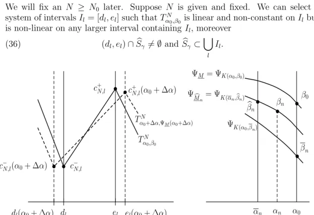
We will fix an N ≥ N0 later. Suppose N is given and fixed. We can select a system of intervalsIl = [dl, el] such thatTαN0,β0 is linear and non-constant onIl but is non-linear on any larger interval containing Il, moreover
(36) (dl, el)∩Sbγ 6=∅ and Sbγ ⊂[
l
Il.
dl el
dl(α0+ ∆α) el(α0+ ∆α) c+N,l(α0+ ∆α)
c−N,l(α0+ ∆α)
c+N,l
c−N,l
TαN0,β0
TαN0+∆α,ΨM(α0+∆α)
b
b bb
αn αn α0
βn β0
βn
βbn
ΨM = ΨK(α0,β0)
ΨK(α0,β
n)
ΨMc
n= ΨK(α
n,bβn)
b
b
b b
Figure 4. Illustration for the proofs of Proposition 10 and Theorem 13 The maximality of the intervals Il implies that
(37) TαN0,β0(dl), TαN0,β0(el)∈ {ci :i= 1, . . . , k} and TαN0,β0(dl)6=TαN0,β0(el).
From (36) it follows that
(38) X
l
λ(Il)≥λ(Sbγ).
By using (37) we introduce the notation
(39) c−N,l =TαN0,β0(dl) and c+N,l =TαN0,β0(el).
From (27) and (37) it follows that
(40) |c+N,l−c−N,l| ≥∆c.
An elementary calculation shows that
d
dx(TαN0,β0(x))
=(TαN0,β0)′(x)= β0
α0
γN(x) β0
1−α0
1−γN(x)!N
for anyx∈(dl, el).
(41)
During the rest of the proof the reader might find useful to look every so often at the left half of Figure 4. Also observe that the value of γN(x) is constant on (dl, el). Denote this constant by gl. Using (35) and (36) we obtain
(42) |gl−γ|< δ1.
By topological conjugacy of Tα,ΨM(α) and Tα0,β0 if we changeα ∈[α1, α2] then the system of maximal intervals of monotonicity ofTα,ΨM(α)is not changing in number and only endpoints of these intervals vary in a Lipschitz continuous way. This means that we can consider the intervals [dl(α), el(α)], α ∈[α1, α2] and the absolute value of the slope of Tα,ΨN
M(α) on these intervals will be for anyx∈(dl(α), el(α))
d
dx(Tα,ΨN M(α)(x))
= ΨM(α) α
gl
·
ΨM(α) 1−α
1−gl!N
= (ΨM(α))N · 1 α
gl
· 1
1−α
1−gl!N
= (s(α, gl))N. (43)
By (34) and (35) we have
(44) s(α0+ ∆α, gl)< s(α0, gl) + 1
2∆α∂1s(α0, gl), that is
s(α0, gl)
s(α0+ ∆α, gl) > 1
1 + 12∆α∂s(α1s(α0,g0,gl)
l)
= 1
1− 12∂1s(αs(α00,g,gl)l)
|∆α| >1 + 1 2
∂1s(α0, gl) s(α0, gl)
· |∆α|. (45)
Using α1 +1−α1 ≥2, (30), (34), (45) and Bernoulli’s inequality (s(α0+ ∆α, gl))N < (s(α0, gl))N
1 + 12∂1s(αs(α00,g,gl)l)
|∆α|N
< (s(α0, gl))N
1 +N · 14|bγ(α0)−γ|(α1 + 1−α1 )|∆α| < (s(α0, gl))N 1 + N2|bγ(α0)−γ||∆α|. (46)