Conditions for Inference Invariant Rule Reduction in FRBS by combining rules with identical consequents
Jayaram Balasubramaniam
Department of Mathematics and Computer Sciences, Sri Sathya Sai Institute of Higher Learning
Prasanthi Nilayam, A.P. -515134, India jbala@ieee.org
Abstract: Following the wide spread usage of Fuzzy Systems, Rule Reduction has emerged as one of the most important areas of research in the field of Fuzzy Control. Many rule reduction methods have been proposed in the literature and can be broadly classified into Lossless or Lossy with respect to the inference, based on whether the outputs of the original and the reduced rule bases are identical or not. In a typical Multi-Input-Single-Output fuzzy system the number of rules far exceeds the number of fuzzy sets defined on the output domain. This suggests that the rule base can be partitioned into sets of rules, each set being mapped to a single consequent fuzzy set. In this paper, we investigate the conditions on the inference operators employed in a fuzzy system that enable “lossless” merging of rules with identical consequents.
After briefly surveying the many techniques that have been proposed towards reducing the number of rules, we propose a general framework for Inference in Fuzzy Systems and then propose some sufficiency conditions on this general framework that give us a class of Fuzzy Systems that allow lossless rule reduction of the type mentioned above. We then explore these conditions in the setting of Fuzzy Logic. We find that R- and S-implications play a very critical role. We give examples from the above class of Fuzzy Systems. In this study we apply the above technique only on rules whose antecedents and consequents are fuzzy sets.
Keywords: Fuzzy Systems, Rule Reduction, Residuated Implications, Strong Implications, Fuzzy Inference.
1 Introduction
Following the wide spread usage of Fuzzy Systems, Rule Reduction has emerged as one of the most important areas of research in the field of Fuzzy Control. It is well known that an increase in the number of input variables and/or the number of mem- bership functions in the input domains quickly lead to a combinatorial explosion in the number of rules. On the other hand the number of output/consequent fuzzy sets remains a constant and is usually far less than the number of rules. This suggests that the rule base can be partitioned into sets of rules, each set being mapped to a single consequent fuzzy set. Thus the rules, though with different antecedents, but with identical consequents can be merged into a single rule. But such merger of rules, though reduces the number of rules may not be lossless, i.e., the inference obtained from the original rule base and the reduced rule base for a given input
may not be identical. In this paper, we investigate the conditions on the inference operators employed in a fuzzy system that enable ”lossless” merging of rules with identical consequents. This provides us with a class of Fuzzy Systems in which the antecedents of the rules with identical consequent can be combined to reduce the number of rules in an inference invariant manner.
In section 2 we give a brief survey of the various rule reduction techniques pro- posed in the literature. In section 3 we propose a general framework for Inference in Fuzzy Systems and in section 4 we give sufficiency conditions on the inference framework that ensure lossless rule reduction of the type mentioned above. In sec- tion 5 we explore each of these conditions in the setting of Fuzzy Logic. In section 6 we give a few examples from the above class of SISO Fuzzy Systems that satisfy the above sufficiency conditions.
2 Rule Reduction as an Issue
2.1 Rule Reduction Techniques in the Literature
For an n-input Multi-Input Single-Output (MISO) fuzzy system, with nimember- ship functions defined on each of the input domains Xi(i = 1,2, . . . ,n), we have m = n1×n2×. . .×nn =Qn
i=1nirules. Thus an increase in the number of input variables and/or the number of membership functions in the input domains quickly lead to a combinatorial explosion in the number of rules.
The several approaches taken towards Rule Reduction in Fuzzy Systems can be classified into the following categories:
• Selection of important rules that contribute significantly to the inference.
• Elimination of redundant rules based on some criteria.
• Merger of rules that share some common property.
2.1.1 Rule Reduction while Building a Fuzzy Rule Base
While trying to build a minimal fuzzy system, the authors in [52, 63] have em- ployed Genetic Algorithm (GA) or GA-type optimisation to eliminate redundant rules and/or identify important or significant rules.
In [44] the authors have converted a linear fuzzy system in which the growth of the parameters with respect to inputs is exponential to an equivalent non linear fuzzy system in which their growth is linear. Works have also appeared that reduce the number of rules by reducing the number of input variables through Mathematical Fusion or through Symbolic Fusion, which involves the use of multi-dimensional fuzzy sets. In [70] a fuzzy binary box tree data structure has been proposed. In [43] the authors have designed a Fuzzy Logic Controller (FLC) based on Variable Structures techniques to be assured of Stability. They have reduced the number of rules from mn to mn, where there are n input domains and m fuzzy sets on each domain.
2.1.2 Rule Reduction in an existing Fuzzy Rule Base
Towards reducing the number of rules in an existing fuzzy rule base, L.T. Koczy and Hirota [51] reduced a dense rule base to sparse rule base, containing the essential information in the original rule base, and all other rules were replaced by the In- terpolation Algorithm that can recover them to a certain accuracy prescribed before reduction.
Following the Selection of significant rules or elimination of redundant rules, Rule Reduction has been addressed in [46,48,52] using GA and Evolutionary Al- gorithms, in [61,79,82] using Orthogonal Transformations, in [13] using Singular Value Decomposition, in [72] using Linear Matrix Inversion. [66] employs a Simi- larity Measure to prune the rules.
In [67] the authors use a similarity measure to merge rules with fuzzy an- tecedents and/or consequents that are similar to each other above a specified thresh- old. Their main stated intention is the reduction in number of fuzzy sets used in the model.
In cases where coupling effects between different inputs are small, the design of an MISO fuzzy system has been reduced to that of designing a set of SISO fuzzy systems, in a decentralised fashion, each SISO fuzzy system being designed for a pair of input-output variables. Many approaches based on the approximation or de- composition of multi-dimensional fuzzy relations into two-dimensional ones have been studied [19,47]. In [41] the conditions for reducing multi-dimensional fuzzy relations into two-dimensional ones are studied for systems using max-min compo- sition operator. However, such approximation may lead to unsatisfactory results if some peculiarities of the process are neglected.
In hierarchical fuzzy controllers introduced in [62] the number of rules increase linearly with the number of system inputs, but the decision of where the different variables are to be put in the hierarchy is often a difficult process.
2.2 Need for Lossless Rule Reduction Techniques
Many of the rule reduction methods in the literature give rise to an approximation error, i.e., the inference obtained from the original rule base and that obtained from the reduced rule base may not be the same.
In [14] Baranyi et al, discuss the trade offbetween Approximation Accuracy and Complexity. See also [50] for a discussion on the trade offbetween computa- tion time and precision. Thus the approximation accuracy achieved should not be sacrificed in the process of complexity reduction. All these necessitate a study on rule reduction techniques that are lossless with respect to inference.
2.2.1 Lossless Rule Reduction Techniques in the literature
A few of the rule reduction techniques that are lossless are listed below. We define
”lossless” in the sense that, the inference obtained from the original rule base and that obtained from the reduced rule base is identical.
In [64] an enhanced two-level Boolean Synthesis methodology is employed, where in, a given fuzzy rule with fuzzy connectives is mapped to a corresponding expression with boolean connectives, with each input fuzzy set being given a label.
The method seeks to reduce the number of connectives employed in the antecedents of the rule. In [45] the authors in order to apply Karnaugh maps for rule reduction represent the linguistic values on a domain as 0 or 1. Though the reduced rule base can infer ”sensibly” even if the original rule base were incomplete, if the output is identical in rules where one or more antecedents are different the method does not merge these rules and thus the rule reduction is incomplete.
In [22] the authors represent a Fuzzy System as a Fuzzy Inference Graph and try to minimise the number of nodes - rules - by a two step process. Again the rule reduction is incomplete since non-interacting antecedents are not combined even though their outputs are identical and also it is lossless only for the min implication operator.
In [23] the authors have proposed a novel, though much debated [24, 25, 30, 59], rule configuration called the Union Rule Configuration, wherein the growth in number of rules is only linear instead of exponential, but the proposed method is applicable only if there is monotonicity or ordering among inputs and member- ship functions and a one-one correspondence between input and output membership functions.
In [49] the author follows a similar approach as ours, that of merging rules with identical consequents by proposing new fuzzy operations where certain properties of regular fuzzy operations have been either relaxed or not imposed.
In [16] Baranyi et al., discuss both exact and non-exact reduction methods using Singular Value Decomposition methods, where by removing only the zero-Singular values one obtains lossless rule reduction and in the case when all Singular values below a threshold are discarded, the error bounds for some special types of fuzzy systems are also given in [11, 12, 80, 81]. Also [14, 15, 17, 18] discuss complexity reduction in Fuzzy Rule Bases using SVD. [13, 69, 82] give an excellent review of rule reduction techniques based on Orthogonal Transformations and discuss their goodness.
2.3 Our Approach towards Lossless Rule Reduction
The approach we take towards Lossless Rule Reduction is to merge rules with iden- tical consequents even with different antecedents. We do not propose any new fuzzy operations to this end, but obtain some conditions that the different operators em- ployed in a fuzzy inference system should satisfy. Also the final reduced rule base, obtained by employing our method, will contain only as many rules in the rule base, as there are output membership functions that featured in the original rule base. If there are n input domains and m input fuzzy sets in each domain the total number of rules that give a complete rule base is mn. The best theoretical limit, so far, of a re- duced rule base is mn [43]. With our method it reduces to k , where k is the number of output fuzzy sets that featured in the original rule base, and typically k≪m.
3 A General Framework for Inferencing in Fuzzy Sys- tems
First we give some preliminaries on Fuzzy Logic Operators that will be required in the rest of this work. As usual we will denote by I the unit interval [0,1].
3.1 Fuzzy Logic Operators
Definition 1 ([37], Definition 1.1, Pg 3). A Negation N is a function from I to I such that:
• N(0)=1; N(1)=0;
• N is non-increasing.
A negation N is called strict if in addition N is strictly decreasing and con- tinuous. A strong negation N is a strict negation N that is also involutive, i.e., N(N(x))=x, ∀x∈I.
Definition 2 ([34] Definition 2.1 Pg 6). A t-norm T is a function from I2 to I such that∀a, b, c∈I,
• T (a,1)=a,
• T (a,b)=T (b,a),
• T (a,T (b,c))=T (T (a,b),c),
• T (a,b)≤T (a,c) whenever b≤c.
Definition 3 ([34] Definition 3.1 Pg 10). A t-conorm S is a function from I2to I such that∀a, b, c ∈I,
• S (a,0)=a,
• S (a,b)=S (b,a),
• S (a,S (b,c))=S (S (a,b),c),
• S (a,b)≤S (a,c) whenever b≤c.
Definition 4 ([34] Definitions 6.1 Pg 17 & 6.11 Pg 18). A t-norm T is said to be
• Continuous if it is continuous in both the arguments;
• Archimedean if for each (x,y)∈(0,1]2there is an n∈Nwith x(n)T <y, where x(n)T =T (x,· · ·,x
| {z }
n times
);
• Strict if T is continuous and stricly monotone, i.e., T (x,y)<T (x,z) whenever x>0 and y<z;
X 0
1 1
0
X 0.4
B
0.4 ∧ B
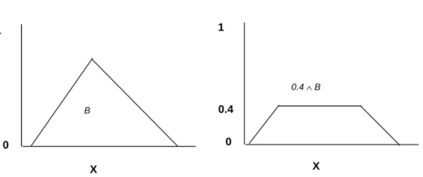
Figure 1: Fuzzy Set B (left) and the fuzzy set 0.4∧B (right)
• Nilpotent if T is continuous and if each x ∈ (0,1) is such that x(n)T = 0 for some n∈N.
Definition 5. If B : X → I, a ∈ I, and R is any binary operator on I, i.e., R : I×I → I, then R(a,B) is a fuzzy set on X, i.e., R(a,B) : X → I, defined as R(a,B)(x)=R(a,B(x)),∀x∈X.
Remark 1. Thus R can also be seen as R : I×F(X)e →F(X)- wheree F(X) denotese the set of all fuzzy sets on X. For example if R(a,b)=min(a,b) then in Figure 1 we have B ∈ F(X) and R(0.4,e B) = min(0.4,B) =0.4∧B ∈ F(X),e i.e.R(0.4,B)(x) = min(0.4,B(x))= 0.4∧B(x), for all x∈X.
Definition 6. If A,B : X→I, and R is any binary operator on I, i.e., R : I×I→I, then R(A,B) is a fuzzy set on X, i.e., R(A,B) : X → I, defined as R(A,B)(x) = R(A(x),B(x)),∀x∈X.
Remark 2. Thus R can also be seen as R : F(X)e ×F(X)e → F(X)- wheree F(X)e denotes the set of all fuzzy sets on X.
X 0
1
A B
(a) Fuzzy Sets A and B
X 0
1
A v B
(b) Fuzzy Set A∨B
Figure 2: Fuzzy Sets A and B
For example if R(a,b)=max(a,b) then in Figure 2(a) we have A,B∈F(X) aree fuzzy sets on X and Figure 2(b) gives A∗=R(A,B)=max(A,B)=A∨B∈F(X).e
Definition 7 ([37] Definition 1.15, Pg 22). A function J : I2 → I is called a fuzzy implication if it has the following properties:
J(p,r)≥J(q,r) i f q≥p, (J1)
J(p,r)≥J(p,s) i f r≥s, (J2)
J(0,r)=1, ∀r∈I, (J3)
J(p,1)=1, ∀p∈I, (J4)
J(1,0)=0. (J5)
The following are the two important classes of fuzzy implications well-estab- lished in the literature:
Definition 8 ([37] Definition 1.16, Pg 24). An S-implication JS,N is obtained from a t-conorm S and a strong negation N as follows:
JS,N(a,b)=S (N(a),b),∀a,b∈I. (1) Definition 9 ([37] Definition 1.16, Pg 24). An R -implication JTis obtained from a t-norm T as its residuation as follows:
JT(a,b)=S up{x∈I : T (a,x)≤b},∀a,b∈I. (2) R- and S-implications satisfy (J1) - (J5). Tables 1 and 2 list few of the well- known S-implications and R-implications, respectively.
Name S (a,b) N(a,b) JS,N(a,b) Dienes max(a,b) 1−a max(1−a,b) Reichenbach a+b−ab 1−a 1−a+ab Lukasiawicz min(1,a+b) 1−a min(1,1−a+b)
Table 1: Some of the well known S-implications with their corresponding t-conorms
t-norm T (a,b) Implication JT(a,b)
Lukasiawicz max(0,a+b−1) Lukasiawicz min(1,1−a+b)
Mamdani min(a,b) Godel
( 1, if a≤b b, otherwise
Larsen min(1,a+b) Goguen
( 1, if a≤b b/a, otherwise Table 2: Some of the well-known R-implications and their corresponding t-norms
3.2 Fuzzy If-Then Rules
A linguistic statement ”x is A” is interpreted as the variable x taking the linguistic value A. For example, if x denotes ”Temperature” (on a suitable domain), then it can assume the following linguistic values A, viz., high, more or less high, medium, cool, very cold, etc. Each of the linguistic values (say cool) is represented by a fuzzy set on the domain X of the linguistic variable x, i.e., A : X → I. The shape of the graph of the function represents the concept (say high temperature). The concept of high temperature is again context-dependent. For example, high temperature (fever) for a human being is different from the high temperature in a blast furnace, and accordingly the domain of the linguistic variable is selected.
A Fuzzy If-Then rule is of the form
If x is A Then y is B, (3)
where x,y are variables and A,B are linguistic expressions/values assumed by the linguistic variables. For example,
”If x (temperature) is A (High) Then y (Pressure) is B (Low)”
The above is an example of a SISO rule. A Two-Input Single-Output rule is of the form
R1: If x is A and y is B Then z is C,
where again A,B,C are linguistic values taken by the linguistic variables x,y,z over their respective domains.
3.3 Di ff erent Stages in the inferencing of a Fuzzy System
Let us consider the following system of m fuzzy if-then rules:
R1 : I f x1is A11, . . . ,xnis A1nT hen y is B1
...
Rj : I f x1is A1j, . . . ,xnis AnjT hen y is Bj (4) ...
Rm : I f x1is Am1, . . . ,xnis Amn T hen y is Bm
where Aij ∈ F(Xe i) for i =1,2, . . . ,n are the antecedent fuzzy sets over the n non- empty domains X1,X2, . . . ,Xn. For j = 1,2, . . . ,m, Bj can be a fuzzy set on the non-empty output domain Y, i.e., Bj ∈ F(Y), as in the case of a Mamdani Fuzzye System, or Bj ∈ Y as in the case of a constant-output Takagi-Sugeno-Kang Fuzzy Systems.
In the following we propose a general framework for Inference in Fuzzy Rule Based Systems that captures the working of both the established models of Fuzzy Systems - TSK and Mamdani models of Inference. Towards this end, a Fuzzy Sys- tem can be seen to consist of the following 5 stages:
3.3.1 Fuzzifier
If the given input is a crisp number x∈X, it is fuzzified to get a fuzzy setX on thee corresponding input space X, i.e., C : X → F(X), where C(x)e =X. Thus given ae vector of crisp points x=[x1,x2, . . . ,xn], where xi ∈ Xi, for every input space Xi, we get a vector of Fuzzy sets X=[fX1,fX2, . . . ,fXn]. The often used [40,79] Singleton Fuzzifier of a crisp number x is given as
e X(y)=
( 1 if y=x (S F∗) 0 otherwise
Remark 3. It can be readily seen that the above stage of ”Fuzzifier” is the reverse of ”Defuzzification” - wherein we obtain a crisp number from a fuzzy set (See 3.3.6 below). Though in many actual implementations of Fuzzy Systems a crisp value is directly given as input, the above stage has been added for generality. Also many times the input given to a fuzzy system is not precise owing to many types of obser- vation errors. For example, a reading from a sensor that becomes an input for the controlling fuzzy system may be inherently imprecise due to instrument errors. In such cases a fuzzy set about the reading may be a more realistic input. In this paper, crisp inputs are identified with their fuzzified version as given by (S F∗).
3.3.2 Matching
The input fuzzy sets (fX1,fX2, . . . ,fXn) are matched against their corresponding if-part fuzzy sets in each of the rule antecedents in the Fuzzy System, i.e.
M :F(Xe i)×F(Xe i)→I (5) where M(Aij,Xei)=aijfor AijandXei∈F(Xe i), j=1, . . . ,m.
A few matching functions used in the literature are given later in section 5.4.1.
3.3.3 Combining
In a multi-antecedent fuzzy system, the various matching degrees aijof the n input fuzzy sets to the antecedent of the jthfuzzy if-then rule are combined to give the ”fit values”µj,
µ: In→I (6)
whereµ(a1j, . . . ,anj)=µj, j=1,2, . . . ,m.µcan be any t- or t-conorms (see Section 3.1).
3.3.4 Rule Firing
The combined valueµjfires the rule consequent or the output fuzzy set Bjof the jth rule. This Bj can be a fuzzy set on Y,i.e.,Bj ∈ F(Y), or a value in Y, i.e.,Be j ∈ Y.
Thus we have
f : I×Z →Z (7)
• When Z = F(Y) - the set of all fuzzy sets on the output domain Y, i.e.,Be j ∈ e
F(Y), f (µj,Bj)= fj∈F(Y) and is defined as f (µe j,Bj(y))= fj(y),∀y∈Y
• When Z=Y, the output domain itself, i.e., Bj∈Y, then fj∈Y and is defined as f (µj,Bj)= fj.
Usually, f =π, the product, is commonly employed when Bj ∈Y ⊆R, while a t-norm or any Fuzzy Implication Operator (Section 3.1) is the prefered choice if Bj∈F(Y).e
3.3.5 Aggregation of Individual Inferences:
The fired output fuzzy sets (or crisp real numbers) fj, j = 1,2, . . . ,m are then aggregated to obtain the final inferred fuzzy set (or crisp real number)
g : Zm→Z (8)
where again
• If Z=F(Y), the infered output set g( fe 1, . . . ,fm)=B∈F(Y). One can use anye of the fuzzy logic operators, t- or t-conorms, to obtain B∈F(Y).e
• If Z =Y ⊆Rthen the Weighted Average or the Weighted Sum are the com- monly used aggregation operators for g.
3.3.6 Defuzzification
When Z = F(Y), g( fe 1, . . . ,fm) = B ∈ F(Y) and we need to defuzzify B - a fuzzye set on Y - to a single value b∈Y, using an appropriate defuzzification method h as follows:
h :F(Y)e →Y (9)
The Centre of Area or the Mean of Maxima methods [42, pp. 336 - 338] are the most widely used Defuzzification methods.
The different stages and the corresponding mappings capturing their actions are given in Table 3.
3.4 Di ff erent Models of Fuzzy System in the literature
Following are the two most established models of Fuzzy Systems:
Fuzzifier: eX=C(x) C : X→F(X)e
Matching: aij=M(Aij,Xei) M :F(Xe i)×F(Xe i)→I Combining: µj=µ(a1j, . . . ,anj) µ: In→I
Firing: fj= f (µj,Bj) f : I×Z→Z,Z=F(Y) or Ye Aggregation: B=g( f1, . . . ,fm) g : Zm→Z
Defuzzification: b=h(B) h :F(Y)e →Y Table 3: Different stages of a Fuzzy System
3.4.1 Mamdani Fuzzy System
E.H. Mamdani and S. Assilian [57] proposed the first type of Fuzzy Rule Based Systems. The rules in a Mamdani Fuzzy System are specified linguistically both for antecedents and consequents. Given a vector of crisp inputs x′=[x′1,x2′. . . ,x′n], where x′i ∈ Xi, the final output fuzzy set B on Y for the fuzzy rule base in (4) is obtained as follows:
B(y) =Wm j=1{[Vn
i=1aij]∧Bj(y)},∀y∈Y (10) where aij=Aij(x′i).
Though the Mamdani model is usually used with crisp inputs, it can handle both crisp and fuzzy inputs. In the case of a fuzzy inputs, say x1 is A1, . . . ,xn is An, where Aiis a fuzzy set on the domain Xi, the final output fuzzy set B on Y for the fuzzy rule base in (4) is given by (10), but with aijgiven by (11)
aij=maxx∈Xi{min(Aij(x),Ai(x))} (11) Also in the case of a crisp input, the crisp input can be singleton fuzzified by (SF*) (Section 3.3.1) into a fuzzy set and can be given as an input to the fuzzy system. Thus given a vector of crisp inputs x′ =[x′1,x′2, . . . ,x′n], where x′i ∈ Xi, for every input space Xi, we get a vector of fuzzy inputs X = [fX1,fX2, . . . ,fXn].
It can be easily seen that if instead of the crisp inputs x′i, if their correspond- ing singleton fuzzified inputs are given, i.e., Ai = Xei are inputs, aij = Aij(x′i) = maxx∈Xi{min(Aij(x),Ai(x)} = maxx∈Xi{min(Aij(x),Xei(x)}. Thus we can always con- sider an input for the Mamdani model of fuzzy system to be fuzzy, with the under- standing that any crisp input is singleton fuzzified according to (SF*) and (10) can be employed with (11).
Let the Matching Function maxx∈X{min(A(x),B(x))} of two fuzzy sets A,B : X → I be denoted by M1(A,B). Now, comparing the inference in (10) to the dif- ferent stages in Section 3.3, it can be seen that M =M1, µ=∧,f =∧,g=∨and Z =F(Y).e
3.4.2 Takagi - Sugeno - Kang Fuzzy System
Instead of working with the linguistic rules of the kind employed in Mamdani Fuzzy Systems, Takagi and Sugeno [71] proposed a new model based on rules whose an- tecedent is composed of linguistic variables and the consequent is represented by a real function of the input variables. TSK model differs from the Mamdani model both in the form of their rules and the inference operators used. If in the case of Mamdani model of a SISO fuzzy system a fuzzy rule has the form (3)
I f x is A T hen y is B
where A and B are fuzzy sets on X and Y, respectively, then in the case of the TSK model the rules have the form (12)
I f x is A T hen y=b(x) (12)
and the input is a crisp value for x. Their conclusion contains the real valued func- tion b(x) and not a fuzzy set. This function can be non-linear, although usually linear functions are applied. Then the TSK rules have the form:
I f x is A T hen y=px+q (13)
where the input is a crisp value for x and p,q are constants. In general the rules of a SISO and MISO TSK fuzzy systems are of the form given by (14) and (15), respectively.
Rj : I f x is AjT hen y =bj(x) (14) Rj : I f x1is A1j, . . . , xnis Anj T hen y =bj(x) (15) for j=1, . . . ,m and the input vector x′=[x′1,x′2, . . . ,x′n] and each xi′is a crisp value in Xifor i=1, . . . ,n.
Let us again consider a fuzzy rule base of m rules of the form (15) and a vector of crisp inputs x′=[x′1,x′2, . . . ,x′n], where x′i ∈ Xi, be given. In the TSK model of fuzzy systems, the final crisp output is obtained as the Weighted Sum of ”fit values”
and the rule consequents as given in (16).
F(x′)= Xm
j=1
µj(x′)·bj(x′) (16)
whereµj(x′)= Πni=1aij= Πni=1Aij(x′i)=A1j(x′1)·A2j(x′2)·. . .·Anj(x′n).
As in Section 3.4.1, by taking the singleton fuzzified crisp input vector x′, as given by (SF*), it can be seen that, if Ai = Xei are inputs, aij = Aij(x′i) = maxx∈Xi{min(Aij(x),Ai(x)}=maxx∈Xi{min(Aij(x),Xei(x)}. Thus again one can always consider the singleton fuzzified fuzzy setXeiof a crisp input x′ias being the input for a TSK model of fuzzy system. Also product is the antecedent combiner, i.e.,µ=Q. Though the product between the ”fit value” of the given input to the antecedents of
rule j,µj(x′) and its consequent bj(x′) is an effect of the Weighted Sum aggregation employed and is not a rule connective, per se, one can perhaps consider it such so that f =πfor the TSK model in the above framework, i.e., f : I×Z → Z is such that f (µj(x′),bj(x′)) =µj(x′)·bj(x′), where Z =Y ⊆ ℜ, the actual domain of the output fuzzy sets.
Now, comparing the inference in (16) to the different stages in Section 3.3, it can be seen that M=M1, µ=π,f =π,g= Σand Z=Y ⊆ ℜ.
From the above two sections, it is clear that the different stages in the inference of an output, given an input, in a fuzzy system can be mapped to different functions capturing the actions performed at every stage.
Definition 10. A model of Inference in a fuzzy system is given by the quintuple Q = {M, µ,f,g,Z}where M, µ,f,g are the corresponding operators of the above framework and Z is the domain of consequents of the rule.
Thus Mamdani Model of inference in a fuzzy system is defined as the quintuple QM = {M1,∧,∧,∨,F(Y)}e while the TSK model of inference in a fuzzy system is given by QT S K = {M1,Q,Q,P,Y ⊆ ℜ}. We do not consider the fuzzifier stage since a crisp input to the fuzzy system can be thought of as a singleton fuzzified input fuzzy set using (S F∗). Table 4 summarises the above discussion, whereQ= Product,P=Sum,∨=max,∧=min.
Name/Type M µ f g Fuzzifier Z
TSK M1 Q Q Σ S F∗ Y ⊆ ℜ
Mamdani M1 ∧ ∧ ∨ S F∗ F(Y)e
Table 4: M, µ,f,g and Z for the different models of fuzzy systems in Section 3.4
3.5 A Rule Reduction Technique for a Class of Fuzzy Systems
More often than not, the number of fuzzy sets, k, defined on the single output domain Y, is typically much less than the number of rules m, i.e., k≪m . This suggests that the antecedents of more than one rule lead to the same consequent. To eliminate this redundancy, we propose a new type of off-line rule reduction where the rules with the same consequent but different antecedents are merged into a single rule. Then we will have only as many rules as there are output membership functions, in fact only those that are part of the original fuzzy system.
The issue involved here is that despite the merging of the above rules, there should be no loss of inference, i.e., the inference obtained from the original rule base and that obtained from the reduced rule base should be identical. This necessitates the functions M, µ,f and g to possess some properties. These are explored in the next section.
Remark 4. Also in the rest of the paper, we will only consider fuzzy rules (SISO or MISO, as the case may be) of the type where both the antecedents and consequents
are fuzzy sets on their respective domains. The inputs may be crisp or fuzzy. In the case of crisp inputs, we will consider their fuzzified version as obtained using (S F∗) on the input.
4 Conditions on the General Framework for Lossless Rule Reduction
The rule reduction procedure we propose is an offline procedure, i.e., from the given original rule base we club the rules with same consequent, but different antecedents, to produce new rules to replace old rules. In this, section we determine the structure of the antecedents of the newly formed rules. The following theorem gives sufficient conditions that the operators of the above proposed framework should satisfy to obtain lossless or inference invariant rule reduction by combining antecedents of rules that have identical consequents.
4.1 The Restrictions on g, f, µ and M :
Theorem 1. Let a model of inference in a fuzzy system be defined by Q = {M, µ,f,g,Z = F(Y)}, where Y is the output domain. The following conditionse on the operators M, µ,f and g are sufficient to ensure inference invariant rule re- duction, by combining antecedents of rules that have identical consequents, in any MISO fuzzy system:
There exist operators g,og,oµ which are commutative and associative binary operators on I and for any a,b,a1,a2,b1,b2 ∈ I, A1,A2,A which are fuzzy sets defined on an input domain X and C∈F(Y),e
g[ f (a,C),f (b,C)]= f (a ogb,C) (17) µ(a1,b1) ogµ(a2,b2)=µ(a1oµa2,b1oµb2) (18) M(A1,A) oµM(A2,A)=M(A1oµA2,A) (19) Remark 5. In the LHS of (19) oµis a binary operator on I while in the RHS of (19) oµis the extension of oµto fuzzy sets on X (See Definition 6 and Remark 2 in Section 3.1).
Proof. Without loss of generality, let us take a 2-input 1-output fuzzy system con- sisting of three rules, where X1 and X2 are the input domains and Y the output domain. Consider the fuzzy system given by the following rules, written in a sim- plified form:
R1 : A1,B1→C
R2 : A2,B2→C (20)
R3: A3,B3→D
where A1,A2,A3are fuzzy sets on X1; B1,B2,B3are fuzzy sets on X2and C,D are fuzzy sets on Y.
Let us consider the inference in the above MISO - fuzzy system in the presence of an input, say ”x1 is A and x2is B”, which is represented as X =(A,B), where A∈F(Xe 1) and B∈F(Xe 2). The MISO inference from the original rule base (20) is given as:
g{ f [µ(M(A1,A),M(B1,B)),C], f [µ(M(A2,A),M(B2,B)),C],
f [µ(M(A3,A),M(B3,B)),D]} (21) Letting µ(M(A1,A),M(B1,B)) as a andµ(M(A2,A),M(B2,B)) as b we have from (17), with g being associative,
(21) = g{g{f [µ(M(A1,A),M(B1,B)),C], f [µ(M(A2,A),M(B2,B)),C]}, f [µ(M(A3,A),M(B3,B)),D]}
= g{f [µ(M(A1,A),M(B1,B)) ogµ(M(A2,A),M(B2,B)),C],
f [µ(M(A3,A),M(B3,B)),D]} (22) Again letting M(Ai,A)=ai∈I,M(Bi,B)=bi∈I, i=1,2, we have using (18) and (19)
(22) = g{f [µ(M(A1,A) oµM(A2,A), M(B1,B) oµM(B2,B)),C],
f [µ(M(A3,A),M(B3,B)),D]} (23)
= g{f [µ(M(A1oµA2,A),M(B1oµB2,B)),C],
f [µ(M(A3,A),M(B3,B)),D]} (24) Thus the rule base in (20) can be reduced to the following rule base containing just two rules:
R∗1 : A1oµA2,B1oµB2→C (25) R3 : A3,B3→D
It can be easily seen that for a given input X =(A,B), the inference obtained from the reduced rule base (25) under the given model of inference Q is identical to
(24).
The above requirements on the general framework give us a class of Fuzzy Sys- tems that allow lossless rule reduction by combining rules with same consequent.
5 Analysis of the Requirements for Lossless Rule Re- duction
In this section, we explore each of the above conditions for Lossless Rule Reduction in the setting of Fuzzy Logic operators.
5.1 Conditions on g, o
gand o
µIn this study we consider only continuous t-norms and t-conorms for g,ogand oµ, which are by definition both commutative and associative. This enables us to extend them to functions from Into I in the case of n-input domains.
5.2 On the Equation (17)
Typically in a Fuzzy System f (the rule firing operation) is interpreted either as a t-norm, for example Mamdani’s min, or a Fuzzy Implication operator. In this work we investigate the solution of (17) both with f as a Fuzzy Implication Operator and as a t-norm. We explore equation (17) in the following way:
• Fix f to be in a specific class of Fuzzy Implications or any t-norm and vary g and hence ogover conitnuous t-norms and t-conorms.
In this study, we consider the two most established and well studied families of Fuzzy Implication Operators, viz., R- and S-Implications. (See Definitions 8 and 9 in Section 3.1).
When f is fixed in (17), g and og are taken to be any S/T-norms, we have the following 4 possibilities:
f (T (p,q),r)=S ( f (p,r),f (q,r)) (26) f (S (p,q),r)=T ( f (p,r),f (q,r)) (27) f (T1(p,q),r)=T2( f (p,r),f (q,r)) (28) f (S1(p,q),r)=S2( f (p,r),f (q,r)) (29) 5.2.1 f =J a Fuzzy Implication
Fixing f to be any Fuzzy Implication J, we get the following four equations from the above:
J(T (p,q),r)=S (J(p,r),J(q,r)) (30) J(S (p,q),r)=T (J(p,r),J(q,r)) (31) J(T1(p,q),r)=T2(J(p,r),J(q,r)) (32) J(S1(p,q),r)=S2(J(p,r),J(q,r)) (33) Recently with f = J interpreted as an R- or an S-implication and g = S , an t-conorm and og=T , a t-norm, Trillas and Alsina [76] have investigated (30) and proven the following:
Theorem 2. An S- or an R-implication J satisfies (30) iffS =max and T =min.
In [7] the authors have proven the following Theorem 3 concerning equation (31) obtained by letting f = J to be an R- or an S-implication and og = S , an t-conorm and g=T , a t-norm,
Theorem 3. An S- or an R-implication J satisfies (31) iffS =max and T =min.
Also we have the following result:
Lemma 1. For no Fuzzy Implication J, t-norm T (t-conorm S , respectively) do equations (32) ((33), respectively) hold.
Proof. Let p =1,q =r=0. Then using the property of t-norms, T (1,0) =0 and (J3), we have that,
LHS o f (32) = J(T1(1,0),0)=J(0,0)=1 RHS o f (32) = T2(J(1,0),J(0,0))=T2(0,1)=0
LHS=RHS implies that 1=0, which is absurd. Similarly, that (33) does not have a solution can be seen by again fixing p=1,q=r=0.
5.2.2 f =T a t-norm
In [76] it is also shown that (30) does not hold for the Mamdani’s Minimum f = J =∧and the Larsen’s Product f = J =Qoperators. That (26) and (27) do not hold when f is any t-norm T can be easily seen by taking p = r = 1 and q = 0.
Thus fixing f =T to be a t-norm,we need to consider only the equations (28) and (29) which become:
T (T1(p,q),r)=T2(T (p,r),T (q,r)) (34) T (S1(p,q),r)=S2(T (p,r),T (q,r)) (35) We have the following theorems:
Theorem 4. (34) is valid iffwhen T1≡T2 =min.
Proof. Claim: T1≡T2on I×I.
Let r=1. Then∀p,q∈I, we have LHS of (34)=T (T1(p,q),1)=T1(p,q)
RHS of (34)=T2(T (p,1),T (q,1))=T2(p,q)=LHS of (34)∀p,q∈I iffT1≡T2. Now, let p=q=1,r∈I. Then
LHS of (34)=T (T1(1,1),r)=T (1,r)=r.
RHS of (34) =T1(T (1,r),T (1,r)) = T1(r,r)=r, ∀r ∈ I iff T1 = min, the only
idempotent t-norm.
Theorem 5. (35) is valid iffwhen S1 ≡S2=S and T distributes over S .
Proof. Claim: S1≡S2on I×I.
Let r=1. Then∀p,q∈I, we have LHS of (35)=T (S1(p,q),1)=S1(p,q)
RHS of (35)=S2(T (p,1),T (q,1))=S2(p,q)=LHS of (35)∀p,q ∈I iffS1≡S2. Thus the equation (35) becomes
T (S (p,q),r)=S (T (p,r),T (q,r)) (36)
which is true iffT distribuites over S .
Corollary 1. (36) is true if S =max.
5.3 On the Equation (18)
Continuing along the same vein, we have investigated the generalised bisymmetry equation (18)
µ(a1,b1) ogµ(a2,b2)=µ(a1oµa2,b1oµb2) involving og, µand oµ, with a1,a2,b1,b2 ∈I.
Definition 11. A function B : [a,b]2→[a,b] is said to be bisymmetric if B(B(x,y),B(u,v))=B(B(x,u),B(y,v)), ∀x,y,u,v∈[a,b].
For a comprehensive coverage on Bisymmetry Equations refer [1 - 4, 74]. Also [38,39] list many results on bisymmetry equations on the unit interval. Allowing og, µand oµto be t- and t-conorms, we get the following 8 possible cases in all, which for convenience we have grouped into two sets:
Group 1
T1(T2(a1,b1),T2(a2,b2))=T2(T3(a1,a2),T3(b1,b2)) (37) S1(S2(a1,b1),S2(a2,b2))=S2(S3(a1,a2),S3(b1,b2)) (38)
Group 2
T1(S (a1,b1),S (a2,b2))=S (T3(a1,a2),T3(b1,b2)) (39) T1(T2(a1,b1),T2(a2,b2))=T2(S (a1,a2),S (b1,b2)) (40) T1(S1(a1,b1),S1(a2,b2))=S1(S2(a1,a2),S2(b1,b2)) (41) S1(T (a1,b1),T (a2,b2))=T (S2(a1,a2),S2(b1,b2)) (42) S1(S2(a1,b1),S2(a2,b2))=S2(T (a1,a2),T (b1,b2)) (43) S1(T1(a1,b1),T1(a2,b2))=T1(T2(a1,a2),T2(b1,b2)) (44)
We show that only 2 of the above 8 equations, the ones belonging to Group 1 have solutions, while the rest of the equations belonging to Group 2 do not have solutions as given by the following theorems, the proofs of which can be found in the Appendix.
Theorem 6. If T1,T2and T3 are any t-norms then the equation (37) obtained by letting og=T1, µ=T2and oµ=T3in (18) is valid iffT1≡T2 ≡T3on I2.
Theorem 7. If S1,S2and S3are any t-conorms then the equation (38) obtained by letting og=S1, µ=S2and oµ=S3in (18) is valid iffS1≡S2≡S3on I2. Theorem 8. The equations belonging to Group 2 do not have solutions.
5.4 On the Equation (19)
In this section, we investigate equation (19), namely, M(A1,A) oµM(A2,A)=M(A1oµA2,A)
where M is a matching function that compares two fuzzy sets on the same domain, i.e., M : F(X)e ×F(X)e → I, with oµ a t- or t-conorm, in which case we get the following equations (45) and (46):
T [M(A1,A),M(A2,A)]=M(T (A1,A2),A) (45) S [M(A1,A),M(A2,A)]=M(S (A1,A2),A) (46) 5.4.1 A few Matching functions existing in the literature
Below we list a few of the matching functions commonly employed in the literature.
• Zadeh’s Sup-min : M1(A,A′)=maxxmin(A(x),A′(x))
• Magrez - Smets’ Measure [56]:M2(A,A′) = maxxmin(A(x),A′(x)) , where A(x) is the negation of A(x).
• Sup-T : M3(A,A′)=maxxT (A(x),A′(x)) , where T is any t-norm.
• Sup-T-N:M4(A,A′)=maxxT (A(x),A′(x)).
• Inf- max :M5(A,A′)=minxmax(A(x),A′(x)).
• Inf - max- N: M6(A,A′)=minxmax(A(x),A′(x)).
• Inf-S : M7(A,A′)=minxS (A(x),A′(x)) , where S is any t-conorm.
• Inf - S - N: M8(A,A′)=minxS (A(x),A′(x)).
Note: M3and M4(M7and M8) are generalisations of M1and M2(M5and M6), respectively, while M5,M6,M7and M8are duals of M1,M2,M3and M4.
The proofs of the following results can be found in the Appendix.
Theorem 9. M1,M2,M3and M4satisfy equation (46) iffS =max.
Theorem 10. M5,M6,M7and M8satisfy equation (45) iffT =min.
Remark 6. M1,M2,M3 and M4 (M5,M6,M7 and M8) do not satisfy (45) (resp.
(46)) since there does not exist any t-conorm S (resp. t-norm T) such that S (minxax,minxbx) = minxS (ax,bx) (such that T (maxxax,maxxbx) = maxxT (ax,bx)). We refer the readers to [20, 21] for the corresponding proofs.
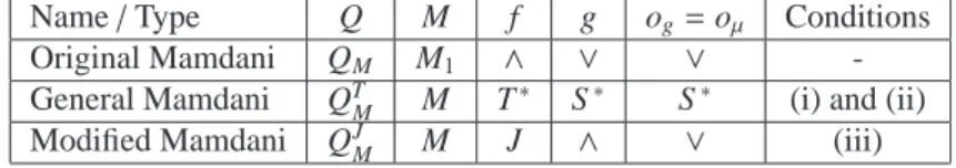
Combining the results of section 5.1 - 5.4, we get the following table - Table 5 - of operators available for equations (17),(18) and (19), where JS,JR denote S- and R-implication, while T and S denote a t-norm and t-conorm, respectively.
f g og µ oµ Conditions Examples of M
JS or JR ∨ ∧ ∧ ∧ - M5,M6,M7,M8
JS or JR ∧ ∨ ∨ ∨ - M1,M2,M3,M4
T ∧ ∧ ∧ ∧ - M5,M6,M7,M8
T S S S S T dist over S M1,M2,M3,M4; S =∨ Table 5: Table of operators for (17),(18) and (19) to be satisfied
6 Examples of a few Fuzzy Systems from the above class
In this section we show how the results from Section 5 can be applied to particular models of inferencing in Fuzzy Systems. For throughout this section, we consider the following SISO fuzzy system with 3 rules as given in (47).
R1: A1→B
R2: A2→B (47)
R3: A3→C
where A1,A2,A3 are fuzzy sets on X; B,C are fuzzy sets on Y and→ is any rule firing operation relating the antecedent to the consequent.
6.1 Mamdani Model of Inference in Fuzzy Systems
Consider the following set of m Single-Input Single-Output (SISO) fuzzy if-then rules of Mamdani type:
I f x is AjT hen y is Bj, j=1,2,· · ·,m
where Ai,Biare fuzzy sets on the input and output domains X,Y, respectively. From Section 3.4.1, we know a Single-Input Single-Output (SISO) Mamdani type Fuzzy System has the final output fuzzy set B given by
B(y) =Wm
j=1{[Aj(x)∧Bj(y)},∀y∈Y (48) which corresponds to QM={M1,na,∧,∨,F(Y)}.e
Remark 7. Since in the case of SISO rule base, the antecedent combinerµdoes not play a role we have indicated it as Not Applicable - na - in QM.
6.1.1 Lossless Rule Reduction in Mamdani Model of Inference in SISO Fuzzy Systems
Theorem 11. Inference Invariant Rule Reduction is possible in Mamdani Model of Inference, in the case of SISO fuzzy rules, by combining the antecedents of rules that have identical consequent.
Proof. We know that f - the rule firing operator - is the t-norm min in (48). In the presence of an input, say x is A, denoted as X = A, we have from (48), the final output fuzzy set B′is given by
B′(y) = [M1(A1,A)∧B]
∨[M1(A2,A)∧B]
∨[M1(A3,A)∧C] (49)
¿From (49) by the distributivity of∧over∨we have (50), B′(y) = {[M1(A1,A) ∨(M1(A2,A)]∧B}
∨[M1(A3,A)∧C] (50)
= [M1(A1∨A2,A)∧B]
∨[(M1(A3,A)∧C] (51)
= [M1(A∗1,A)∧B]∨[(M1(A3,A)∧C] (52) We know from Theorem 9 that M1(A1,A)∨M1(A2,A) = M1(A1 ∨A2,A), using which we obtain (51) from (50). In (52) A∗1=A1∨A2, which is again a fuzzy set on X, by Definition (6) and Remark 2.
Thus instead of the SISO fuzzy rule base of 3 rules (47), the following reduced rule base with two rules can be used, without any loss of inference for a given input, while employing the Mamdani Model of Inference.
R1 : A∗1→B
R3 : A3→C (53)
6.2 General Mamdani Model of Inference in Fuzzy Systems
A slight generalisation of the Mamdani model of inference can be seen as follows:
Let QTM = {M,na,T∗,S∗,F(Y)}e denote a General Mamdani Model of Inference where T∗is any t-norm that distributes over the t-conorm S∗. Then the following can be easily shown as above:
Theorem 12. Inference Invariant Rule Reduction is possible in Mamdani Model of Inference, in the case of SISO fuzzy rules, by combining the antecedents of rules that have identical consequent, if the Matching function M is such that
S∗[M(A1,A),M(A2,A)]=M(S∗[A1,A2],A). (54) In the case S∗ =max, the matching function M, among others, can be one of M1,M2,M3,M4.
6.3 Modified Mamdani Model of Inference in Fuzzy Systems
By a Modified Mamdani Model of Inference we refer to the following quintuple QJM = {M,na,J,∧,F(Y)}, where M is any Matching function and J is either ane R- or an S-implication. In this model of inference an Implication Operator J is employed to relate the antecedent and the consequent of the fuzzy rules. The final output fuzzy set B in QJMfor a SISO rule base is given by
B(y) =Vm
j=1{[Aj(x)→Bj(y)},∀y∈Y (55) where→is either an R- or an S-implication.
Recently Li et al [54,55] have shown that the above Modified Mamdani Model of Inference in Fuzzy Systems with R- or S-implications for the rule firing operation and with Trapezoidal or Triangular membership functions are Universal Approxi- mators both in the case of SISO and MISO fuzzy systems. (In the case of MISO systems the antecedent combiner µ = ∧). These considerations make Modified Mamdani Model of Inference very attractive. In this section we show that lossless rule reduction is possible in Modified Mamdani Model of Inference in the SISO case.
6.3.1 Lossless Rule Reduction in Modified Mamdani Model of Inference in SISO Fuzzy Systems
Theorem 13. Inference Invariant Rule Reduction is possible in Modified Mamdani Model of Inference, in the case of SISO fuzzy rules, by combining the antecedents of rules that have identical consequent, if the Matching function M obeys (56).
M(A1,A)∨M(A2,A)=M(A1∨A2,A). (56) Proof. Let us now interpret f - the rule firing operator - as an R- or an S-implication in (55). Let us again consider the above SISO fuzzy system of 3 rules as given in