The Pseudooperators in Second Order Control Problems

(1)

The Pseudooperators in Second Order Control Problems

Márta Takács

Institute of Intelligent Engineering Systems, John von Neumann Faculty of Informatics, Budapest Tech

Bécsi út 96/B, H-1034 Budapest, Hungary takacs.marta@nik.bmf.hu

Abstract: This paper deals with the control of a dynamic system where the gains of the conventional PD controller are previously chosen by fuzzy methods in such a way as to obtain the optimal trajectory tracking. The gain factors are determined by solving fuzzy equations, and based on the sufficient possibility measure of the solution. It will be shown, that the rule premise for the given system input in fuzzy control system may also determine the possibility of realizing a rule. This possibility can be used for verifying the rule and for changing the rule-output, too. This leads to the optimization of the output. When calculating the possibility value the possible functional relation between the rule-premise and rule-consequence is taken into account. For defining the rule of inference in Fuzzy Logic Control (FLC) system special class of t-norm is used. The proposed fuzzy logic controller uses the functional relation between the rule premises and consequences, and the special class of pseudo-operators in the compositional rule of inference.

Keywords: FLC, fuzzification of the linear equations, PD controllers, pseudo-operators

1 Introduction

There is a question that arises during the studying of fuzzified functions: what are those practical problems where given beside certain fuzzified function parameters, an approximation can be provided to other unknown but also fuzzy-type function parameters. If a scruple, linear function relationship is observed, the fuzzification problem of the

y e K e

K_p + _d = (1)

type law of the PD-type controller emerges.

The conventional linguistic FLC uses fuzzified quantities e,e(error and error change) as inputs and y as output. The rules of this system are

(2)

Y is then E is and E is

if e e y

where E,Eand Y are linguistic terms, whose can be NB(negative big), NM(negative medium), NS(negative small), ZE(zero), PS(positive small), PM(positive medium), PB(positive big). Fuzzy membership functions cover linguistic terms. The scaling and normalization of parameters domains are made by experts.

The input variables of a dynamic system to be controlled can be the error (e), which is the difference between the desired and the actual output of the system and the errorchange (e). In a typical PD controller using these variables the y output is determined by the control law given by the equation (1), where the control gains Kp,Kd also could be modified during the operation in order to bring the system to be controlled into a desired state. There types of FLCs are called tuning-type controllers. In the literature there are indications regarding the solution of this problem. Some soft computing based techniques have been published for the on-line determination of these gains[1].

In further explanation a possible way for tuning these parameters is given, to achieve an efficient system-performance. The architecture of the proposed controller can be seen in Fig. 1. The conventional PD controller and the Fuzzy Logic Controller (FLC) use the same e,e input variables and the FLC also uses the output y of the PD controller (this is required because of the linear relationship in K_pe+K_de= y). The FLC gives two crisp outputs, the gains Kp ,Kd, to the PD controller that calculates the new y by using these gains and e,e as inputs. The rules of the FLC are given in the the form of:

(

isE and isE and isY

)

then

(

isKp and isKd

)

if e e y K_p K_d (2)

where E,E,Y,Kp,Kd are linguistic terms, which can be for example N(negative), Z(zero), P(positive). Fuzzy membership functions cover linguistic terms. The scaling and normalization of parameters domains are made by experts.

The performance of the propose self tuning controller has been evaluated. For this purpose a second order differential equation has been chosen. The results serves to show the effects of the operators used in the rules of inference as well as the effects of the generalized t-norms.

The theoretical background of the membership functions of the linguistic terms is given, and the applied generalized t-norms and their generator functions are summarized, based on the general theoretical publication [2], [3]. A theoretical interpretation of possibility measure of the rule realization is given using the same generator function as by definition of the membership functions and applied t- norm. The functional dependence used to determine the possibility of the rule plays a very important role. It can be used for the rule base construction, and for

(3)

the inference mechanism as well by narrowing the linguistic rule consequence.

With these narrowing rule consequences a modified FLC model can be constructed, where the rule consequences are surfaces above the Kp,Kd plane.

In the paper a method which using the functional relationship betweenK_p,K_d,e,e,y parameters is presented, that creates the rule base on one hand, and furthermore uses this functional dependence in the inference mechanism too.

Figure 1

The architecture of the proposed controller

Figure 1 illustrates how such a tuning FLC can be integrated into the system. The conventional PD controller and the FLC has the same e,e as inputs and the tuning FLC also uses the output y of the conventional controller (this is required because of the linear relationship in (1)). The FLC gives two crisp outputs to the PD controller that calculates a new y by using these gains and e,e as inputs.

Following the procedure of FLC construction, contains of steps:

st1 determination of fuzzification strategy st2 the choise of quantities to be fuzzified

st3 fuzzification of these quantities and the rule base construction st4 choosing of inference mechanism

st5 choosing of defuzzification model,

these general steps cover different mathematical procedures depending on the choice of strategy. This paper presents two procedures on an example: a Mamdani-type, in which a novel construction of the rule-base is given, and another one which is said to be possibility-modified and the rule possibilities integrated into the rule outputs.

step input

q ^d + _

de PD

eout

FLC

scaling of

[e,e,y]

scaling of

[K^p,K^d]

system

e ^e

e y q out

q - q ^d = e

q

(4)

2 General Concept

2.1 Special Types of the Fuzzy Numbers

A fuzzy subset A of a universe of discourse X is defined as

( )

{

∈ →[0,1]

}

= x, x x X, :X

A μ μ_A . Denote FX the set of all fuzzy subsets of X.

The characteristic function of A will be denoted by χ_A. If the universe is X = ℜ, and we have a membership function

⎪⎩

⎪⎨

⎧ ⎟⎟ ≠

⎠

⎞

⎜⎜

⎝

⎛ −

= ⁻

0

= if

0

1 if

δ χ

δ δ α

α(x), x , ) g

x ( A

) (

(3) α∈ℜ,δ≥0, then the fuzzy set given by A(x) will be called quasitriangular fuzzy

number with the center α and width δ, and we will recall for it by QTFN(α,δ).

2.2 Pseudo-operators

Generally details about pseudo-analysis and pseudo-operators we can read in [4], [5]and [6].

Pseudo-analysis

The base for the pseudo-analysis is a real semiring, defined in the following way:

Let

[ ]

^a,^b be a closed subinterval of

[

⁻^∞^,^+∞

]

(in some cases semi-closed subintervals will be considered) and let ≺ be a total order on

[ ]

a,b . A semiring is the structure

(

^≺^,^⊕,^⊗

)

if the following hold:

⊕ is pseudo-addition, i.e., a function ⊕^:

[ ] [ ] [ ]

â^,^b × â^,^b → â^,^b which is commutative, non-decreasing (with respect to ≺), associative and with a zero element denoted by 0;

⊗ is pseudo-multiplication, i.e., a function ^⊗^:

[ ] [ ] [ ]

â^,^b ^× â^,^b ^→ â^,^b

which is commutative, positively non-decreasing (x≺y implies y

x z

x⊗ ≺ ⊗ where ^z^∈

[ ]

^a^,^b + ⁼

{

^z^z^∈

[ ]

^a^,^b^,⁰^≺^z

}

associative and for which there exists a unit element denoted by 1.

0 0⊗z=

(

^y ^z

) (

^x ^y

) (

^x ^z

)

x⊗ ⊕ = ⊗ ⊕ ⊗

(5)

Three basic classes of semirings with continuous (up to some points) pseudo- operations are:

(i) The pseudo-addition is an idempotent operation and the pseudo- multiplication is not.

(ii) Semi-rings with strict pseudo-operations defined by a monotone and continuous generator function g:

[ ] [

a,b → 0,+∞

]

, i.e., g-semirings:

( ) ( ) (

^g ^x ^g ^y

)

g y

x⊕ = ⁻¹ + and ^x^⊗^y⁼^g⁻¹

(

^g

( ) ( )

^x^g ^y

)

. (iii) Both operations, ⊕ and ⊗, are idempotent.

More on this structure can be found in [4].

T-norm as the Pseudooperator

Let T: I² → I , (I=[0,1]) be a a t-norm. The t-norm is Archimedian if and only if it admits the representation ^T

( )

^a^,^b ⁼^g⁻¹

(

^g

( ) ( )

^a ⁺^g ^b

)

, where the generator function g: I→ ℜ⁺ is continuous, strictly decreasing function, with the boundary conditions ,g(0)= , ( ) =1 g1 0 and let

( )

( ) ( )

⎪⎩

⎪⎨

⎧

∉

= ⁻ ∈

−

I 0

1 I

1

x x x x g

g (4)

the pseudoinverse of the function g. The generalization of this representation is

( ) (

^p

( )

^p

( ) )

^p

gp a,b g g a g b

T

1

1 +

= ⁻ , (5)

and it can be said, that the T_gpfunction is an Archimedian t-norm given by generator function g^p,p∈

[

1,∞

)

.

t-norms were introduced as binary operations. Since they are associative, they also can be considered as operations with more than two arguments.

(i) The associativity (T2) allows us to extend each t-norm T in a unique way to an n-ary operation by induction, defined for each n-tuple

(

x₁,x₂,...xn

)

∈

[ ]

0,1ⁿ,

(

ⁿ^∈^N^∪

{ }

⁰

)

as ,

1

0

1

=

= i i

T

x ⁱ ⁿ

⁽

ⁿ

⁾

n i i n i

x x x T x x T

x

T

^, ¹^, ²^,...

1

1 1

⎟⎟=

⎠

⎞

⎜⎜⎝

= ⎛ ⁻

=

If, in a specific case, we have

x

₁

= x

₂

= ... = x

_n

= x

, in short, it can be written in the form ( )n

x

T instead of

( )

n

x x x

T , ,... .

(6)

(ii) The fact that each t-norm T is weaker than the minimum TM makes it possible to extend it to a countable infinity operation, putting for each

( )

xi _i_∈_N ∈

[ ]

0,1^N

i n n i i i

x

T

1 1

lim

∞ =

→

∞

=

Note that the limit on the right side always exists, since the sequence

N n i n i

T

x

= ⎟⎟⎠ ∈

⎞

⎜⎜⎝

⎛

1

is non-increasing and bounded from below.

Continuity of the T-norms

In general, a real function of two variables, e.g., with the domain

[ ]

⁰^,¹² may be continuous in each variable without being continuous on

[ ]

⁰^,¹². Triangular norms and conorms are exceptions from this.

Proposition. A t-norm is continuous if and only if it is continuous in its first component, i.e., for each fixed y∈

[ ]

⁰^,¹ the one-place function

( )

^⋅^,y ^:

[ ] [ ]

⁰^,¹ ^→ ⁰^,¹

T , or briefly x→T

( )

x,y is continuous.

Keeping in mind that the only extra property for the t-norm T was the monotonicity, the proposition can be extended for any monotone function F of two variables, which is continuous in both components.

For applications quite often weaker forms of continuity are sufficient.

2.3 FLC Systems

One rule in a FLC system has form: if x is A

( )

x then y is B

( )

y , where x is the system input, y is the system output, ^x^isA

( )

x is the rule-premise, y is B

( )

y is the rule-consequence. A(x) and B(y) are linguistic terms and they can be described by QTFN-s.

For a given input fuzzy set A'

( )

x , in a mathematical-logical sense, the output fuzzy set B'

( )

y , the model of the compositional rule of inference in the Mamdani type controller will be generated with a Generalized Modus Ponens (GMP):

(7)

( ) ( ( ( ) ( ) ) ( ) ) ( ( ) ( ) ) ( )

⎟⎟

⎠

⎞

⎜⎜

⎝

⎛

=

∈

∈ T T Ax,A' x ,B y T supT Ax,A' x ,B y sup

y ' B

DOF X x X

x

(6)

where DOF is the degree of firing value for the rule.

2.4 The Fuzzification of the Linear Equalities

Possibility Logic

In possibility logic the propositions can be true or false, but we do not know exactly their truth value. If we know the truth value of several of them, then we can infer the truth value of more complex terms.

Every proposition p∈P, (where the (P,∨,∧,¬) is a Boolean-algebra) has:

• Possibilistic measure: Poss(p)

• Necessity measure: Nec(p), with the following properties:

• Poss (false)=0=Nec(false)

• Poss(true)=1=Nec(true)

∀p,q∈P , Poss(p∨q)=max(Poss(p),Poss(q))

∀p,q∈P , Nec(p∧q)=min(Nec(p),Nec(q))

∀p∈P , Nec(p)=1-Poss(¬p) The essential consequences are:

max(Poss(p),Poss(¬p))=1 min(Nec(p),Nec(¬p))=0 Nec(p)≤Poss(p).

For us the following properties are important Poss(p∧q) ≤ min(Poss(p),Poss(q)) Nec (p∨q) ≥ max(Nec(p),Nec(q)) For α,β∈I

⎩⎨

⎧

>

+

≤

= +

1 if

Im 0

β α β

β β α

α

is a monotone increasing operation. It is easy to see, that Poss(p∧q) ≥ Nec(p) Im Poss(q).

(8)

Possibility Measure of the Control Law

The e,

e

,y values in (1) are uncertain, so they can be replaced by the quasitriangular fuzzy numbers,

( )

^{( )}

( ) ( )

( )

^e ^{( )} ^,^e

( )

êîsâ

(

^,

)

^type^fuzzy^number

e

number fuzzy type ,

a is e e ,

2 2

1

1 1

1

δ δ δ δ

v v

e e g e

e e

⎟⎟

⎠

⎞

⎜⎜

⎝

= ⎛ −

⎟⎟

⎠

⎞

⎜⎜

⎝

= ⎛ −

−

( )

^{( )} _⎟^⎟

⎠

⎞

⎜⎜

⎝

= ⁻ ⎛ −

3 1

δ yv

g z z

y , y(z) is a (yv,δ₃) type fuzzy number, (δ₁,δ_{2 ,}δ₃>0).

If δ₁,δ_{2 ,}δ₃=0, then ^{e e}

( )

= χev

( ) ( )

^{e e e}, =χev

( )

^e , ^{y z}

( )

= χyv

( )

^z are singletons, given by characteristic functions.

0 1=

⋅

− +K e y e

K_p _d

We can give a (g,p,δ) fuzzification of this equality:

( )

^{( )}

( )

⎟⎟⎟

⎠

⎞

⎜⎜

⎜

⎝

⎛ − −

= ⁻

d q p

v v d v p d

p K K

y e K e K g K K

3 2 1 1

, ,

, δ δ δ

σ

σ(K_p,Kd) is a possibilistic measure of equality

( ) ⁽ ⁾

( )

(

l e e y Kp Kd

) ⁽

Kp Kd

⁾

Q

E , , , , ,χ₀ =σ , , i.e.

(

p d

)

d

pe K e y K K

K

Poss( + = )=σ , .

For fixed Kp,Kd values we have an interpreted term, and σ(Kp,Kd) is the truth value for them in possibility logic. Kp,Kd have to be choosen to provide the maximum value of σ(K_p,Kd) which is equal to 1.

A conventional IF ... THEN rule to determine Kp,Kd in case of given e,

e

,y is the following:

( )

e ANDe

( )

e ANDy

( )

z THENKp

( )

Kp ANDKd

( )

Kd

e

IF .

The possibility of realization of this rule by using these inputs and taking into account the linear relatian between the parametrs (Eq. (1)) results in the modified rule

( ) ( ) ( ) ( )

⎟⎠

⎜ ⎞

⎝

⎛ ⎟

⎠⎞

⎜⎝

⎛

Kd Kd Kp Kp THEN z y AND e e AND e e

IF σ , .

(9)

Possibility and Necessity Measures of the Equation System

If some dynamically not coupled systems, given in Fig. 2 work simultanously then an equation type (1) can be related to each system. The possibility measures of realization of an equation by fixed Kp,Kd is

(

p d

)

d

pe K e y K K

K

Poss( + = )=σ , .

If we have two equations, we have σ₁(K1p,K1d), σ₂(K2p,K2d), and the possibility measure of the simultaneous realization of these equations and simultaneous working of systems by the actual parameter values is

σ((K1p,K1d) ∧ (K_2p,K2d)) ≤min(σ1(K1p,K1d), σ2(K2p,K2d)) and furthermore

σ1((K1p,K1d) ∧ (K2p,K2d)) ≥Nec(K1p,K1d) Im σ2(K2p,K2d)=

( ) ( )

( ) ( ) ( )

( ) ( ( ) )

( ) ( ) ( ( ) )

⎩⎨

⎧

¬

>

¬

≤

⎩ =

⎨⎧

>

+

≤ +

1d 1p 2d

2p 2d

2p

1d 1p 2d

2p

2d 2p 1d

1p 2d

2p

2d 2p 1d

1p

K , K K

, K K

, K

K , K K

, K

K , K K

, K K

, K

K , K K

, K

σ σ

σ

σ σ

σ

if if 0

1 Nec

if

1 Nec

if 0

σ ((K2p,K2d) ∧ (K1p,K1d)) ≥ Nec (K2p,K2d) Im σ2(K1p,K1d) =

=

( ) ( ( ) )

(

⁰

)

^if^if^σ

( )

^σ

( ( ) )

σ σ σ

K , K K , K

K , K K , K K , K

1p 1d 2p 2d

1p 1d 1p 1d 2p 2d

≤ ¬

> ¬

⎧

⎨⎪

⎩⎪

The necessity of the simultaneous realization of these equations is analogously Nec ((K1p,K1d) ∨ (K_2p,K2d)) ≥max(Nec (K_1p,K1d) , Nec(K2p,K2d))

when the Nec (K1p,K1d) and Nec(K2p,K2d) are the given as heuristic necessity measures by experts.

The Possibility Model of the Problem (1)

The membership function of the t-norm of fuzzy sets is defined as follows

( ) ( )

^x ^ν ^x ^T

(

^μ

( ) ( )

^x^,^ν ^x

)

μ ∩ = ∈ FR (7)

The Mamdani type controller applies the rule: if x is μ

( )

^x then y is ν

( )

^y , where x is the system input, y is the system output, ^x^is^μ

( )

^x is the rule-premise,

( )

^y

ν is

y is the rule-consequence. μ(x) and ν(y) are linguistic terms and they can be described by QTFN-s.

(10)

For a given input fuzzy set μ′

( )

^x , in a mathematical-logical sense, the output fuzzy set

ν ′ ( ) y

, will be generated with a Generalized Modus Ponens (GMP).

At every fixed x∈ℜ a T-fuzzification of the function value of the parametric function f(a1,a2,...ak, x) by the fuzzy parameter vector μa=

(

μ₁,μ₂,...μk

)

is a fuzzy set of FR..

The (g,p,δ) fuzzification of a linear equality α_{1 1}x +α₂x₂+ +... α_nx_n =α₀ by the fuzzy vector parameter μa =

(

μ₁,μ₂,...μn

)

(where the coefficients αi are uncertainly parameters, and replaced by μi

(

αi,δi

)

QTFN-s, and the fuzzification of function will be defined by Tgpnorm), is

( ) ( )

( )

^⎟^⎟_⎠

⎞

⎜⎜

⎝

⎛

⋅

− + +

= +

⎟⎟

⎠

⎞

⎜⎜

⎝

⎛

= ⁻ ⋅ ⁻

q n ) n

( q )

(

x diag

x ...

x x g l

x diag

x , g l

x δ

α α α

α δ

σ ¹ α ¹ ¹ ¹ ² ² ⁰ (8)

where

( )

⎪⎪

⎩

⎪⎪⎨

⎧

∞

=

∞

<

⎟ ≤

⎟

⎠

⎞

⎜⎜

⎝

⎛

= ∑

=

p v

max

p v v

,...

v , v

j j p p j

p j n p

1

2 1

1

,

⎪⎪

⎩

⎪⎪

⎨

⎧

−

∞

=

otherwise 1

1

= if

= if 1

p p

p p q

and diag(δ) is a diagonal matrix from elements δ_i. σ(x) will be called possibility measure of equality [2]. All the properties, written in the section 2.2. are necessery for the proof of the propositions above.

Let be Tgp an Archimedian t-norm given by generator function g^p, p∈[1,∞).

The membership function of the t-norm of fuzzy sets is defined as follows

( ) ( )

^x ^ν ^x ^T

(

^μ

( ) ( )

^x^,^ν ^x

)

μ ∩ = ∈ FR (9)

The Mamdani type controller applies the rule: if x is μ

( )

x then y is ν

( )

y , where x is the system input, y is the system output, ^x^is^μ

( )

^x is the rule-premise,

( )

y ν is

y is the rule-consequence. μ(x) and ν(y) are linguistic terms and they can be described by QTFN-s.

For a given input fuzzy set ^μ^′

( )

^x , in a mathematical-logical sense, the output fuzzy set

^ν ^′ ( ) ^y

, will be generated with a Generalized Modus Ponens (GMP).

At every fixed x∈ℜ a T-fuzzification of the function value of the parametric function f(a1,a2,...ak, x) by the fuzzy parameter vector μa=

(

μ₁,μ₂,...μk

)

is a fuzzy set of FR..

(11)

Let EQ be a non-fuzzy equality relation on universe. The T-fuzzification of EQ is a fuzzy set on FR× FR

( ) ( )

(

^x^, ^y

)

^sup^T

( ( ) ( )

^x^, ^y

)

^sup^T

( ( ) ( )

^x^, ^x

)

Q E

x y

x

ν μ ν

μ ν

μ = =

= (10)

The (g,p,δ) fuzzification of a linear function l

( )

α,x =α₁x₁+α₂x₂+...+αnxn by the fuzzy vector parameter μa =

(

μ₁,μ₂,...μn

)

(where the coefficients αi are uncertainly parameters, and replaced by QTFN

(

αi,δi

)

,and the fuzzification of function will be defined by Tgp norm), is given in [4].

The (g,p,δ) fuzzification of a linear equality α₁x₁+α₂x₂+...+α_nx_n =α₀ by the fuzzy vector parameter μa =

(

μ₁,μ₂,...μn

)

is:

( )

( ) ⁽ ^{)( )}

( ) ( )

( )

^⎟^⎟_⎠

⎞

⎜⎜

⎝

⎛

⋅

− + +

= +

⎟⎟

⎠

⎞

⎜⎜

⎝

⎛

= ⋅

=

−

q n ) n

( q )

(

a a

x diag

x ...

x x g l

x diag

x , g l

x

x , l , x , l Q E

δ

α α α

α δ

σ α

μ χ μ

0 2

2 1 1 1 1

0 0

(11)

σ(x) will be called possibility measure of equality [2],[3].

3 Construction of the Mamdani-type FLC for Control Law, Example

st1 Let us chose a Mamdani-type linguistic model for the problem (1).

st2 e,e,y quantities are uncertain, fuzzified, and comprise the FLC and the rule-inputs. Kp, Kd are also uncertain, fuzzified but they comprise the outputs. The rule type for the scaling of the gain papameters Kp, Kd is

(

isE and isE and isY

)

then

(

isKp and isKd

)

if e e y K_p K_d

shortly

( )

^e^then^K ^K

( )

ôrîfÊ Ê ^Y

( )

^e^then^K

( )

Y E E

if ∩ ∩ _p∩ _d k ∩ ∩ k .

(Details see in [4])

st3 Experts can provide those

[

−Le,Le

][

,−Le,Le

]

intervals where e,e quantities exist. For simplification and generalization of the problem these

[

−Le,Le

][

,−Le,Le

]

intervals are normalized and transformed into interval [-1,1]. During the scaling operation e,e receive 77 linguistic terms, there being determined by (3) type fuzzy numbers, for example

(12)

⎪⎩

⎪⎨

⎧ ⎟⎟ ≠

⎠

⎞

⎜⎜

⎝

⎛ −

= ⁻

0

= de if

0 de E if

1

), e (

de , e g e

) e (

ec

) c (

χ e

\

e NB NM NS ZE PS PM PB NB NB NB NB NM NM NS ZE NM NB NB NM NM NS ZE PS NS NB NM NM NS ZE PS PM ZE NM NM NS ZE PS PM PM PS NM NS ZE PS PM PM PB PM NS ZE PS PM PM PB PB PB ZE PS PM PM PB PB PB

Table 1

These 49 possibilities would increase seven times if the y quantity was normalized and scaled likewise. It should be noted, however, that e,e,y quantities are not independent from each other. The relationship generally used by experts in such controllers, (see Table 1 for the y quantity), can be applied for completing input parameters into the rule. Finally we have 49 different rule inputs. The scaling of y is the same on normalized interval [-1,1].

For the rule outputs also linguistic terms are defined which are obtained within the domain of Kp,Kd by scaling. The

[

−LK_p,LK_p

]

,

[

−LK_d,LK_d

]

intervals and the scaling are determined by experts. For the given E,E,Y the suitable Kp,Kd ruleoutputs are chosen based on experience meta-rules or tiresome experimental work.

In our case the Kp,Kd output fuzzy domains will be determined as such for which the possibility of law (1) is the greatest, in case of given E,E,Y.

First let us assign linguistic terms to Kp,Kd (like by e,e,y) on

[

−LK_p,LK_p

]

,

[

−LK_d,LK_d

]

interval. The possible K_pisK_pand K_disK_d (i.e.

Kp∩K_d) domain-number is 49.

Define the possibility measure:

( )

^{( )}

[ ]

^⎟^⎟^⎟

⎠

⎞

⎜⎜

⎜

⎝

⎛

⋅

−

= ⁻ +

q T d p

c c d c p d

p diag( ) K ,K ,

y e K e K g

K , K

1

σ δ (12)

for each rule-premise . The possibilistic rule is defined as follows:

( )

e then σ

(

K_p,K_d

)

or if E E Y

( )

e then σ

( )

k Y

E E

if ∩ ∩ ∩ ∩

(13)

In principle, any Kp∩Kd intersection can be assigned as output to the rule-premise, but in our case the one with the greatest possibility is used, i.e.

( ) ( )

(

k ^Kijk

)

,^i,^j⁼^1,...7.

min max max) j max, i ( poss

k j ,

i ⎟

⎠

⎜ ⎞

⎝

⎛ ∩

= σ (13)

is the greatest. The suitable output is Kimax,jmax

( )

^k^.

{ }

(

^Kp∩^Kd∈^Kij,i,j=¹,²...⁷

)

. So finally the obtained rule-base is:

if e is N & e is Z & y is N then kp is Z & kd is P if e is N & e is P & y is Z then kp is Z & kd is Z if e is Z & e is N & y is N then kp is P & kd is Z if e is Z & e is Z & y is Z then kp is Z & kd is Z if e is Z & e is P & y is P then kp is N & kd is Z if e is P & e is N & y is N then kp is Z & kd is Z if e is P & e is Z & y is P then kp is Z & kd is N if e is P & e is P & y is P then kp is Z & kd is P st4 The inference mechanism is the GMP.

( ) ( )

( )

K

( )

Y E E

K n the Y

E E if

o i

i i

k e

∩

(14) where ^Ei∩^Ei∩^Yi

( )

e is the really, actual FLC input.

st5 The defuzzification can be one of the generally accepted methods. The outputs of the j-th rule are ^KPj

( )

^{and KD} ⁽ ⁾

o

j

Kp o Kd , the rule base output is obtained by summarizing all of them:

( ) ( ) ( ) ( )

d

o ... j , d j o p o ... j , p j

o K max KP K ,KD K max KD K

KP

10 2 1 10

2

1 =

= =

= (15)

The FLC outputs after defuzzification are:

( ) ( )

p o Kp

p o Kp p

p sum K

K K

sum K

KP

⋅KP

∗ =

,

( ) ( )

KD KD

d o Kp

d o Kd d

d sum K

K K

sum K

⋅

∗ =

(16)

The modified system of rules consists of if E∩E∩Y

( )

^e then K

( )

^k ∩σ

( )

^k

(14)

rules.

Thus the output in case of one rule is as follows:

( ) ( ) ( )

( )

K

( )

Y E E

K n the Y

E E if

poss i

i i

k e

k k e

∩

∩ σ

(17)

( ) ( )

K_poss k = K_poss K_p,K_d is a surface above the Kp,Kd plaine, and it is described with a matrix. The summarized rule base output is computed with max too, as in (11).

The defuzzification process is:

( ) ( )

K

sum K K

Sum K

K

sum K K

Sum K

p

Kp p

o p

Kp o

p

d Kd

o

d d

T

Kp o

d

∗ = ∗

∗

=

∗ KP

KP

KD KD

, , where the ∗ operation is

multiplication of matrixes KPô, KDô and vectors Kp,Kd , and the Sum is summa of all the elements of matrixes KPô, Kdô.

st6 The defuzzification can be one of the generally accepted methods.

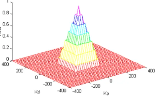
Example 1

Let be

[

−^LK_p^,^LK_p

]

=

[

−^LK_d^,^LK_d

]

=

[

−^400,⁴⁰⁰

]

.

For rule-premise if e isPM and eisNM and yis ZE from the rule-base, and for g(t)=1−t_, q=∞ the possibility measure is:

( )

^{( )}

(

¹

)

^'

3 1

3 0 2 3

2

1

⎟⎟

⎟

⎠

⎞

⎜⎜

⎜

⎝

⎛

+ +

⋅

⎟−

⎠

⎜ ⎞

⎝⎛−

⋅ +

⋅

= ⁻

d p

K K

g K , σ K

(15)

Figure 2

( )

⁴⁴ =¹

= poss , max)

j max, i (

poss (see Figure 2)

Figure 3

Figure 3 shows the chosen rule-consequence. The complete rule is

ZE is and ZE is n the ZE is and NM is and PM is

if e e y K_p K_d .

3.1 Modified Mamdani Model

The modified model differs from the one described in the previous part, in which instead of using only possibility measure based or only linguistic outputs their intersection is used. Therefore, the modified system of rules consist of

( )

^e

( )

^k ∩σ

( )

^k

∩

∩E Y then K E

if rules. Thus the inference mechanism is as

follows:

(16)

( ) ( ) ( ) ( )

K

( )

Y E E

K n the Y

E E if

poss i

i i

k e

k k e

∩

∩ σ

Example 2: For the same parameter-choice from Example 1. Kposs

( )

^k form is shown on the Figure 4. Consequently, the linear dependence of the parameters are not used only in the rule base construction andverification but in the inference mechanism as well, thus narrowing the linguistic rule consequence. Bearing in mind that the rule output is two-dimensional, geometrically the

K

_poss

( ) k

forms are more complex nevertheless, a suitable defuzzification procedure can be found.

Figure 4

Conclusions

The (1) type law of the PD-type controller, as linear function relationship, was fuzzified using function-fuzzification theory. The calculation of possibility measure offers new horizons for the rule base construction and verification not only in the case of linear function relationship but also in any general function relationships. Out of the values poss(imax,jmax), the greatest that determined the ^K

( )

^k domain, is in interval [0,1], and as realization measure of the given rule, it is a rule-weighing. So we obtain a narrowing linguistic rule-consequence. A new method for on-line determination of the gains of a PD controller by using a separate new type fuzzy logic controller is given. Based on the linearity of the control law the possibility measure of the rules of the FLC were introduced. The calculation of these possibility measures offers new horizons for the rule base construction. The proposed new FLC model restricts the Mamdani type rule consequences to possibility domain. In order to verify the performance of the proposed controller simulation has been carried out. It was concluded that in case of the application of generalized t-norms and pseudo-operators in the rules and in

(17)

the inference mechanism the new method provide better performance than the conventional type controller.

References

[1] R. R. Yager, D. P. Filev, Essential of FuzzyModeling and Control,Book, New York/John Wiles and Sons Inc./, 1994

[2] M. Kovács, An optimum concept for fuzzified mathematical programming problems,Interactive Fuzzy Optimization, Berlin-Heidelberg-New York/Springer Verlag/, 1991, pp. 36-44

[3] M. Takács, Fuzzy control of dynamic systems based on possibility and necessity measures, Proc., RAAD’96, 5^th International Workshop on Robotics In Alpe-Adria-Danube Region, Budapest, June 1996

[4] Pap, E., (1997), Pseudo-analysis as a mathematical base for soft computing, Soft Computing, 1, pp.61-68

[5] Klement, E. P., Mesiar, R, Pap, E., 'Triangular Norms', Kluwer Academic Publishers, 2000, ISBN 0-7923-6416-3

[6] Fodor, J., Rubens, M., (1994), Fuzzy Preference Modeling and Multi- criteria Decision Support. Kluwer Academic Pub.,1994