3 The invariant tau in the filtered theory

ALBERTOCAVALLO

We introduce a generalization of the Ozsv´ath-Szab´o τ-invariant to links by studying a filtered version of link grid homology. We prove that this invariant remains unchanged under strong concordance and we show that it produces a lower bound for the slice genus of a link. We show that this bound is sharp for torus links and we also give an application to Legendrian link invariants in the standard contact 3-sphere.

57M25, 57M27

1 Introduction

Link Floer homology is an invariant for knots and links in three-manifolds, discovered in 2003 by Ozsv´ath and Szab´o [8] and independently by Jacob Rasmussen [12], in his PhD thesis. It is the homology of a chain complex whose generators are combinatorially defined, and whose differential counts pseudo-holomorphic disks. Grid diagrams are simple combinatorial presentation of links in S³, dating back to the 19^th century. A grid diagram is anl×lgrid of squares,lof which are marked with an Oandlof which are marked with anX. A projection of a link together with an orientation on it can be associated to a grid diagramD. These grids can be used to give a simpler reformulation of link Floer homology, called grid homology. Of course these two homologies are isomorphic, nevertheless grid homology can be easier to study.

In this paper we use the same notation of the book “Grid homology for knots and links” [7]. In this book particular attention is given to two versions of the grid homology of a linkL: thesimply blocked grid homology dGH(L) and thecollapsed unblocked grid homology cGH⁻(L); both these homology groups are invariant under link equivalence. We study a slightly different version of dGH(L). Let us denote withFthe field with two elements; we start constructing a filteredF-complex

GC(D),c ∂b

from a grid diagram D, equipped with an increasingZ-filtrationF and we prove that F induces a filtration in homology, leading to the filtered homology group dGH(L). The latter is not completely unrelated todGH(L) as we see in Section2.

We can extract a numerical invariant from the homology dGH(L), the integer-valued function TL :

Z×Z−→Z>0, with the following properties.

Proposition 1.1 i) The functionT_Lis supported in{1−n, ...,0}×Zand X

d,s∈Z

T_L(d,s)=2ⁿ⁻¹, wherenis the number of components ofL.

ii) IfL^∗ is the mirror of then-component linkLthen

T_L^∗(d,s)=T_L(−d+1−n,−s) for anyd,s∈Z.

iii) If L₁#L2 is a connected sum ofL₁ andL₂ then T_L1#L2 is the convolution product ofT_L1 and TL₂.

arXiv:1512.08778v2 [math.GT] 8 Feb 2018

iv) IfLis a quasi-alternating link then TLis determined by the signature of L.

Moreover, in Section4we prove the following theorem, which is similar to what Pardon proved in [10] for Lee homology. We say that a strong cobordism is a cobordism Σ, between two links L₁ andL₂, such that every connected component ofΣis a knot cobordism between a component ofL₁ and one ofL₂; in particular L₁ and L₂ have the same number of components. Ifg(Σ) =0 thenΣ is a strong concordance.

Theorem 1.2 The functionT is a strong concordance invariant. In other words, if L₁ andL₂ are strongly concordant thenTL₁(d,s)=TL₂(d,s) for everyd,s∈Z.

In Section3 we show that TL(0,s) is non-zero only for one value of s. We call this integer τ(L), and, as the name suggests, it coincides with the classicalτ for knots defined in [8]. More precisely, we prove the following statement.

Theorem 1.3 For ann-component link theτ-set, defined in [7] as -1 times the Alexander gradings of a homogeneous, free generating set of the torsion-free quotient ofcGH⁻(L) as anF[U]-module, coincides with the2ⁿ⁻¹ (with multiplicity) values ofs where the functionT is supported.

For a knot K, where the τ-set is just τ(K), we have that T_K(d,s) is non-zero only for (d,s) = (0, τ(K)).

From Theorem1.2 we know that τ(L) is a strong concordance invariant. Furthermore, it gives a lower bound for the slice genus g₄(L), that is the minimum genus of a compact, oriented, smoothly and properly embedded surface in D⁴ withLas boundary.

Proposition 1.4 For every n-component linkL we have

(1) |τ(L)|+1−n6g₄(L).

We use this lower bound to give another proof that, for the positive torus linkT_q,p, we have (2) g₄(Tq,p)= (p−1)(q−1)+1−gcd(q,p)

2 for anyq6p.

This was already proved by the author in [1] using the Rasmussens-invariant.

Finally, we use τ(L) to prove a generalization of the Thurston-Bennequin number upper bound, given by Olga Plamenevskaya in [11], to n-component Legendrian links. A brief introduction on Legendrian knots and links can be found in [2].

Proposition 1.5 Consider a Legendrian n-component link L of link type L in S³ equipped with the standard contact structure. Then the following inequality holds:

(3) tb(L)+|rot(L)|62τ(L)−n.

Equation (3) gives a lower bound forτ and, using Equation (1), also the following lower bound for the slice genus ofL:

(4) tb(L)+|rot(L)|62g4(L)+n−2,

generalizing a result of Rudolph [13] for knots. In Section 6 we give an example where this bound is sharp. Moreover, Equation (3) can also give an upper bound for TB(L), the maximal Thurston-Bennequin number of a linkL.

Proposition 1.6 For every n-component linkL we have TB(L)62τ(L)−n.

In particular for a quasi-alternating link, since from iv) in Proposition1.1the invariantτ is determined by the signature, we have the following result that Plamenevskaya proved for alternating knots in [11].

Corollary 1.7 IfLis a quasi-alternating link then we have that TB(L)6−1−σ(L).

As we show in Section6, the upper bound in Corollary1.7gives the following proposition.

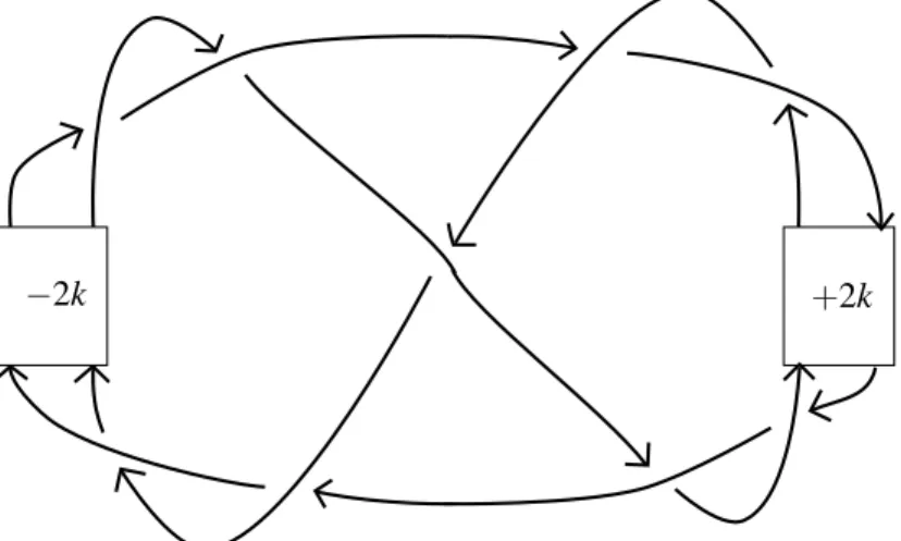
−2k +2k

Figure 1: A diagram ofL^k. For k=0 we have the linkL9^a₄₀.

Proposition 1.8 The links L^k in Figure1are a family of two component links, whose components L^k_i are unknots with linking number zero, such that TB(L^k) is arbitrarily small.

The paper is organized as follows. In Section2we define the filtered chain complexGC(D) and thec homology groupGHd(L). In Section3we introduce the function TL and we prove Proposition1.1.

In Section4we construct maps in homology, induced by a cobordism Σbetween two linksL₁ and L₂ and we use them to prove Theorem1.2and Proposition1.4. In Section5we talk briefly about the filtered version ofcGH⁻(L) and we explain the proof of Theorem1.3. Finally, in Section6we give some applications, including the proof of Equations (2) and (3).

Acknowledgements

The author would like to thank Andr´as Stipsicz for the many helpful conversations and the lots of time spent meeting and discussing mathematics. The author is supported by the ERC Grant LDTBud from the Alfr´ed R´enyi Institute of Mathematics and a Full Tuition Waiver for a Doctoral program at Central European University.

2 Filtered simply blocked link grid homology

2.1 The complex

We always suppose that a link is oriented. We denote byD a toroidal grid diagram that represents an n-component link L. The number grd(D) is the number of rows and columns in the grid. The

X X

X X

(0,0) X (0,5)

(5,0) (5,5)

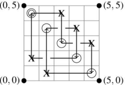
Figure 2: A grid diagram of the positive trefoil knot.

orientation in the diagram is taken by going from the X to the O-markings in the columns and the opposite in the rows. Vertical lines are numbered from left to right and horizontal lines from bottom to top, as shown in Figure2. We identify the boundaries of the grid in order to make it a fundamental domain of a torus; then the lines of the diagram are embedded circles in this torus. Any grd(D)-tuple of pointsxin the grid, with the property that each horizontal and vertical circle contains exactly one of the elements ofx, is called a grid state of D.

Consider the set of theO-markingsO={O₁, ...,O_grd(D)}. We call specialO-markings a non-empty subsetsO⊂Othat contains at most oneO-marking from each component of L, while we call the others normalO-markings. We represent the special ones with a double circle in the grid diagram.

In the paper we usually consider only the case when #|sO|=n, which means there is exactly one special O-marking on each component. We talk about the general case in Subsection 3.2. From now on there are always n special O-markings in a grid diagram, unless it is explicitely written differentely.

We define the simply blocked complex GC(D) as the freec F[V₁, ...,Vgrd(D)−n]-module, where F=Z2Z, over the grid statesS(D)={x₁, ...,x_grd(D)!}.

We associate to every grid state x the integer M(x), called the Maslov grading of x, defined as follows:

(5) M(x)=M_O(x)=J(x−O,x−O)+1 ;

whereJ(P,Q)=X

a∈P

#{(a,b)∈(P,Q)|b has both coordinates strictly bigger than the ones ofa}

with coordinates taken in the interval [0,grd(D)).

Then we have the Maslov F-splitting

GC(D)c =M

d∈Z

GCcd(D)

where GCcd(D) is the finite dimensional F-vector space generated by the elements V₁^l1 ·...·V_m^lmx, withx∈S(D) and m=grd(D)−n, such that

M(V₁^l1 ·...·V_m^lmx)=M(x)−2

m

X

i=1

li =d.

We define another integer-valued function on grid states, the Alexander grading A(x), with the formula

A(x)= M(x)−M_X(x)

2 −grd(D)−n

2 ;

whereM_X(x) is defined in Equation (5), replacing the setOwithX. For the proof thatA(x) is really an integer we refer to Chapter 8 in [7].

Now we introduce an increasing filtration on GC(D) such thatc F^sGC(D)c =M

d∈Z

F^sGCc_d(D)

and where F^sGCc_d(D) is generated over F by the elements V₁^l1 ·...·V_m^lmx with Maslov grading d and Alexander grading

A(V₁^l1 ·...·V_m^lmx)=A(x)−

m

X

i=1

l_i6s.

2.2 The differential

First we take x,y ∈ S(D). The set Rect(x,y) is defined in the following way: it is always empty except whenx andydiffers only by a pair of points, say{a,b}inxand{c,d}iny; then Rect(x,y) consists of the two rectangles in the torus represented by D that have bottom-left and top-right vertices in{a,b} and bottom-right and top-left vertices in{c,d}. We call Rect^◦(x,y) ⊂Rect(x,y) the subset of the rectangles which do not contain a point ofx (ory) in their interior.

The differential∂bis defined as follows:

∂xb = X

y∈S(D)

X

r∈Rect^◦(x,y) r∩sO=∅

V₁^O1(r)·...·V_m^Om(r)y for anyx∈S(D)

where O_i(r) =

(1 ifOi ∈r

0 ifO_i ∈/r. Here {O₁, ...,O_m} is the set of the m = grd(D) −n normal O-markings.

We extend∂btoGCc_d(D) linearly, and we call it∂bd, then again to the whole GC(D) in the followingc way: ∂(Vb ix)=Vi·∂xb for every i=1, ...,m andx∈S(D). Since ∂bkeeps the filtration and drops the Maslov grading by 1 (Lemma 13.2.3 in [7]), we have maps

∂bd,s:F^sGCc_d(D)−→ F^sGCc_d−1(D)

where ∂b_d,s is the restriction of ∂bd to the subspace F^sGCcd(D) ⊂GCcd(D). Furthermore ∂b◦∂b=0 (Lemma 13.2.2 in [7]).

2.3 The homology

We define the homology group GHd_d(D) as the quotient space Ker∂bd

Im∂b_d+1. Moreover, we introduce the subspaces F^sGHdd(D) as follows: consider the projection πd : Ker∂bd → dGHd(D). Since Ker∂bd,s=Ker∂bd∩ F^sGCc_d(D) we say that

F^sdGH_d(D)=πd(Ker∂b_d,s)

for everys∈Z. Ker∂b_d,s⊂Ker∂b_d,s+1 implies that the filtration F descends to homology. We see immediately that eachF^sdGHd(D) is a finite dimensionalF-vector space.

We can extend the filtration F on the total homology GH(D)d =M

d∈Z

GHdd(D) by taking

F^sGH(D)d =M

d∈Z

F^sdGHd(D).

From [7] Chapter 13 we know that the dimension of F^sGHd_d(D) as an F-vector space is a link invariant for everyd,s∈Z, in particular they are independent of the choice of the specialO-markings and the ordering of the markings. Hence we can denote them with F^sdGH_d(L). Furthermore, [7]

Lemma 13.2.5 says that [Vip]=[0] for everyi=1, ...,m and [p]∈dGH(L). This means that each homology class can be represented by a combination of grid states and every levelF^sGH(L) is alsod a finite dimensionalF-vector space.

The homology group dGH_d,s(L) of [7] can be recovered from the complex GC(D) in the followingc way. We denote the graded object associated to a filtered complex C the bigraded chain complex

gr(C),gr(∂) , where

gr(C)d,s= F^sC_d F^s−1Cd

and gr(∂) is the map induced by∂ on gr(C). Then we have that GHd_d,s(L)∼=_F H_d,s

gr

GC(D)c

,gr(∂)b

.

3 The invariant tau in the filtered theory

3.1 Definitions

Since F^s−1GHd_d(L) ⊂ F^sdGH_d(L), and they are finite dimensional vector spaces, we define the function

T_L(d,s)=dim_F F^sGHd_d(L) F^s−1dGH_d(L) which clearly is still a link invariant.

Our first goal is to see what happens to this function T when we stabilize the link L, in other words when we add a disjoint unknot to L. Denote the unknot with the symbol . We claim that

(6) TLt(d,s)=TL(d,s)+TL(d+1,s) for anyd,s∈Z.

Before the proof of Equation (6) it is time for some remarks on filtered chain maps.

Suppose f : (C, ∂) →(C⁰, ∂⁰) is a chain map between two filtered chain complexes overF. We say thatf is filtered of degreetiff(F^sC)⊂ F^s+tC⁰ for everys∈Z.

A filtered chain map induces a map in homology that is filtered of the same degree. This means that f induces a mapf∗:H∗(C)→H∗(C⁰) such that f∗(F^sH∗(C))⊂ F^s+tH∗(C⁰) for anys∈Z.

We say that a linear map F : H∗(C) → H∗(C⁰) is a filtered isomorphism if F is bijective and F(F^sH_∗(C))=F^sH_∗(C⁰) for any s ∈Z. We denote with H_∗(C)∼=H_∗(C⁰) two filtered isomorphic homology groups such that the isomorphism preserves the grading; more excplicitely this means thatF^sHd(C)∼=_F F^sHd(C⁰) for everyd,s∈Z.

Moreover, we can associate to a filtered chain mapf :C → C⁰ the quotient map gr(f) : gr(C)−→gr(C⁰).

We callf a filtered quasi-isomorphism if the map gr(f) induces an isomorphism betweenH_∗,∗(gr(C)) andH∗,∗(gr(C⁰)) that preserves the gradings. We denote with C ∼=C⁰ two filtered quasi-isomorphic complexes.

From Proposition A.6.1 in [7] we have that if there is a filtered quasi-isomorphism between (C, ∂) and (C⁰, ∂⁰) thenH∗(C)∼=H∗(C⁰). While from Proposition A.8.1 in [7] we know thatC ∼=C⁰ if and only if there is a filtered chain homotopy equivalence betweenCandC⁰, providedC andC⁰ are also modules overF[V₁, ...,Vm]. See [7] Chapter 13 and Appendix A for more details.

Finally, we define the shifted complexC[[a,b]]=C⁰ asF^sC_d⁰ =F^s−bCd−a. Now, in order to prove Equation (6), we need the following proposition.

Proposition 3.1 For any linkLwe havedGH(Lt)∼=GH(L)⊗Vd , whereV is the two dimensional F-vector space with generators in grading and minimal level (d,s)=(−1,0)and(d,s)=(0,0).

Proof Take a grid diagram D for L. Then the extended diagram D, obtained from D by adding one column on the left and one row on the top with a doubly-marked square in the top left, represents the link Lt . The circle in the doubly-marked square is forced to be a special O-marking and we can also suppose that there is another specialO-marking just below and right of it, as shown in Figure3.

X z

Figure 3: We call the top-left special O-markingO₀.

LetI(D) denote the set of those generators inS(D) which have a component at the lower-right corner of the doubly-marked square, and letN(D) be the complement ofI(D) inS(D). From the placement of the specialO-markings, we see thatN(D) spans a subcomplexNinGC(D). Moreover, ifc ∂b₁is the

differential inGC(D) andc ∂b2 the one inGC(D) we can express the restriction ofc ∂b1 to the subspace I, spanned by I(D), with ∂b₂+∂bN; this because there is a one-to-one correspondence between elements ofI(D) and grid states inS(D). This correspondence induces a filtered quasi-isomorphism i: (I,∂b2)→GC(D).c

Define a map H:N→I by the formula H(x)= X

y∈I(D)

X

r∈Rect^◦(x,y) O0∈r

V₁^O1(r)·...·V_m^Om(r)y for anyx∈N(D).

We have thatHis a filtered chain homotopy equivalence between (N,∂b₁) and (I,∂b₂), which increases the Maslov grading by one, andH◦∂b_N=0. To see the first claim, we mark the square just on the right ofO₀ withzand we define an operatorHb_z:I→N, which counts only rectangles that contain z. This operator is a homology inverse ofH; this and the second claim can be proved in the same way as in Lemma 8.4.7 in [7]. Those two facts together tell us that the following diagram commutes.

I N

GC(D)c GC(D)[[c −1,0]]

∂b_N

i i◦H

0

Since H is a filtered chain homotopy equivalence, i◦H is a filtered quasi-isomorphism, just like the mapi. Therefore, we can use a filtered version of Lemma A.3.8 in [7] and obtain that the map between the mapping cones

Cone(∂bN)=GC(D)c −→Cone(0)=GC(D)c ⊗V

is a filtered quasi-isomorphism and so the claim follows easily. See also the proof of Lemma 8.4.7 in [7] for other details.

Equation (6) is obtained immediately from Proposition3.1, in fact we have proved thatF^sdGH_d(Lt )∼=F^sGHdd(L)⊕ F^sdGH_d+1(L) for everyd,s∈Zand so it is enough to apply the definition ofT. Now we are able to do some computations. The homology of the unknot can be easily computed by taking the grid diagram of dimension 1, where the square is marked with both X and O. The complex has one element of Maslov and Alexander grading 0; then T(d,s) =1 if (d,s) =(0,0) and it is 0 otherwise.

Using Equation (6) we get the function T of then-component unlink_n: T_n(d,s)=







n−1 k

if (d,s)=(−k,0), 06k6n−1

0 otherwise

.

We can also see this directly from Proposition3.1, in fact we have thatGH(d _n)∼=V^⊗(n−1). Now let us consider a grid diagram D of a link L. The Maslov grading of the elements of S(D) and the differential ∂b are independent of the position of the X’s, once we have fixed the

special O-markings. Since we can always change the X-markings to obtain n, this means that dim_FdGH_d(L)=dim_FdGH_d(_n) for everyd∈Z and the generators are the same. In particular

GH(L)d ∼=_F dGH(_n)∼=_FF²

n−1 and GHd_d(L)∼=_F F(ⁿ⁻¹−d) when 1−n6d60.

From this we have thatGHd₀(L) has always dimension 1 and then we defineτ(L) as the only integer s such that TL(0,s) >0, as we previously said in the Introduction. We remark that for a knot this version ofτ coincides with the one of Ozsv´ath and Szab´o. See the proof of Theorem1.3in Section 5. We also observe that Equation (6) tells that τ(Lt )=τ(L).

3.2 Dropping the special O-markings

In this subsection we study what happens to the homology of the filtered chain complex

GC(D),c ∂b if the grid diagram Dhas less thannspecial O-markings.

Let us considerDa grid diagram for ann-component linkL. The setsO⊂Ocontains at most one O-marking from each component ofL, but we have that #|sO|>1. Denote withm=grd(D)−#|sO| the number of normalO-markings inD. Then we can define our chain complex exactly in the same way as in Section2; on the other hand, the homology dGH(D) is no longer a link invariant, in fact it clearly depends of the choice of the specialO-markings.

Nonetheless, we can show that theF-vector spaceGH(D) is still finite dimensional. Note that thisd is not true if instead we consider the simply blocked homology groupGH(D).d

Proposition 3.2 The homology group GH(D)d , defined as in Subsection 2.3, is F-isomorphic to GH d _#|sO|

, the homology of the unlink with #|sO| components each containing a special O-marking. In particular, we have that

GH(D)d ∼=_F F²

#|sO|−1

and dGHd(D)∼=_F F(^#|sO−d^|−1) when 1−#|sO|6d60.

Proof As we noted before, the group dGH(D) does not depend on the position of theX-marking.

Since we can always change them in a way thatD becomes a diagram for an unlink with a special O-marking on every component, the claim follows from the results in the previous subsection.

Even though in this case the homology is no longer a link invariant, we can still prove the following theorem.

Theorem 3.3 Let us consider two grid diagramsD₁ and D₂ representing smoothly isotopic links L₁ andL₂ such that all the isotopic components both contain or not contain a special O-marking.

Then we have that dGH(D₁) is filtered isomorphic to dGH(D₂) and the isomorphism preserves the Maslov grading. Hence, we can denote the homology group of ann-component linkLwithGHd^O(L) and it depends only on which components of the link contain a specialO-marking.

Proof Lemma 4.1 in [14] tells us that such two grid diagrams differ by a finite sequence of grid moves: reordering of the O-markings, commutations and stabilizations. See Section 3 in [14] for more details. Then it is enough to prove the theorem in the case when D₂ is obtained from D₁ by one of these three moves.

Applying the results in [7] Chapter 5 and 13 we find filtered quasi-isomorphisms for each move and this impliesGH(Dd ₁)∼=GH(Dd ₂).

We use the homology groups dGH^O(L) to define some cobordism maps in Section4.

3.3 Symmetries

3.3.1 Reversing the orientation

If−Lis the link obtained from Lby reversing the orientation of all the components then (7) T−L(d,s)=TL(d,s) for anyd,s∈Z

andτ(−L)=τ(L).

To see this, consider a grid diagram D of L, then it is easy to observe that, if we reflect D along the diagonal going from the top-left to the bottom-right of the grid, the diagram D⁰ obtained in this way represents −L. Hence, we take the map Φ :S(D) → S(D⁰) that sends a grid state x into its reflectionx⁻and now, from Proposition 4.3.1 in [7], we have thatM(x⁻)=M(x) andA(x⁻)=A(x).

This means that Φ is a filtered quasi-isomorphism between GC(D) andc GC(Dc ⁰), since clearly the differentials commute withΦ. This gives thatGHd(−L)∼=GHd(L) and then Equation (7) follows.

3.3.2 Mirror image

For an n-component link L we have that the function T of the mirror image L^∗ is given by the following equation

(8) T_L^∗(d,s)=T_L(−d+1−n,−s) for anyd,s∈Z.

The proof of this relation is similar to the proof of Proposition 7.1.2 in [7]. First, given a complex C with a filtration F, we introduce the filtered dual complex C^∗, equipped with a filtration F^∗ by taking

(F^∗)^s(C^∗)d =Ann(F^−s−1C_−d)⊂(C_−d)^∗ =(C^∗)d for anyd,s∈Z,

where Ann(F^hC_k) is the subspace of (C_k)^∗ consisting of all the linear functionals that are zero over F^hCk.

Second, given a grid diagramDofL, we call

GC(D),f ∂e

the filtered fully blocked chain complex

GC(D),c ∂b

V₁=...=Vm=0 and we also denote withWthe two dimensionalF-vector space with generators in grading and minimal level (d,s)=(0,0) and (d,s)=(−1,−1). We want to prove the following proposition.

Proposition 3.4 dGH(L^∗)∼=GHd^∗(L)J1−n,0K, where the filtration on dGH^∗(L) isF^∗.

Proof LetD^∗ be the diagram obtained by reflectingDthrough a horizontal axis. The diagramD^∗ represents L^∗. Reflection induces a bijection x →x^∗ between grid states for Dand those for D^∗, inducing a bijection between empty rectangles in Rect^◦(x,y) and empty rectangles in Rect^◦(y^∗,x^∗).

Hence, the reflection induces a filtered isomorphism

GC(Df ^∗)∼=GCf^∗(D)[[1−grd(D),n−grd(D)]],

where the shifts are given by the fact that M(x^∗)=−M(x)+1−grd(D) andA(x^∗)=−A(x)+n− grd(D).

Now, from Lemma 14.1.11 in [7], we have the filtered quasi-isomorphism (9) GC(D)f ∼=GC(D)c ⊗W⊗(grd(D)−n)

. Combining these two relations and observing that

(W^∗)⊗(grd(D)−n)∼=W⊗(grd(D)−n)[[grd(D)−n,grd(D)−n]]

leads to the filtered quasi-isomorphism

GC(Dc ^∗)∼=GCc^∗(D)[[1−n,0]].

Proposition3.4 says thatF^sdGH_d(L^∗) ∼= (F^∗)^s

dGH^∗

d−1+n(L) for every d,s ∈ Z. Then we can prove Equation (8):

T_L^∗(d,s)=dim

(F^∗)^s

dGH^∗

d−1+n(L) (F^∗)^s−1

dGH^∗

d−1+n(L)

=dim Ann

F^−s−1GHd_−d+1−n(L)

Ann

F^−sGHd_−d+1−n(L) =

=dim F^−sGHd_−d+1−n(L)

F^−s−1GHd−d+1−n(L) =T_L(−d+1−n,−s).

If we defineτ^∗(L) as the unique integer such that T_L(1−n, τ^∗(L))=1 then we have proved that

(10) τ(L^∗)=−τ^∗(L).

In particular for a knotK, where τ^∗(K)=τ(K), we haveτ(K^∗)=−τ(K). Moreover, we have the following corollary.

Corollary 3.5 Suppose thatLis smoothly isotopic toL^∗. Then, T_L^∗(d,s)=T_L(d,s) for anyd,s∈Z

and so Equation (8) gives that the function TL has a central symmetry in the point ¹⁻ⁿ₂ ,0 . In particularτ^∗(L)=−τ(L) and, for knots,τ(K)=0.

3.3.3 Connected sum

Given two links L₁ andL₂, the function T of the connected sum L₁#L2 is the convolution product of theT functions ofL₁ andL₂; in other words

(11) TL₁#L2(d,s)= X

d=d1+d2

s=s1+s2

TL₁(d₁,s₁)·TL₂(d₂,s₂) for anyd,s∈Z.

This equation is very hard to prove in the grid diagram settings, but it has been proved quite easily using the holomorphic definition of link Floer Homology. In fact Ozsv´ath and Szab´o proved that, if D is a Heegaard diagrams for L andCFL(D) denotes the link Floer complex, there is a filteredd chain homotopy equivalence

CFL(Dd 1)⊗CFL(Dd 2)−→CFL(Dd 1#D2) which gives thatdGH(L₁#L₂)∼=GH(Ld ₁)⊗dGH(L₂). See Section 7 in [8].

We see immediately that the homology and theTfunction ofL₁#L₂ are independent from the choice of the components used to perform the connected sum; moreover the τ-invariant is additive:

τ(L1#L2)=τ(L1)+τ(L2). 3.3.4 Disjoint union

The disjoint union of two links L₁ andL₂ is equivalent to L₁#(L₂t ). Thus by Equation (6) and (11) we have the following relation:

(12) TL₁tL₂(d,s)= X

d=d1+d2

s=s1+s2

TL₁(d1,s₁)· TL₂(d2,s₂)+TL₂(d2+1,s₂)

for anyd,s∈Z,

or in other words: GH(Ld ₁tL₂)∼=dGH(L₁)⊗dGH(L₂)⊗V, whereV is the two dimensionalF-vector space with generators in grading and minimal level (d,s) =(−1,0) and (d,s) =(0,0). We have immediately that

τ(L1tL₂)=τ(L1#L2)=τ(L1)+τ(L2). 3.3.5 Quasi-alternating links

We recall that quasi-alternating links are the smallest set of linksQthat satisfies the two properties:

(1) The unknot is in Q.

(2) Lis inQ if it admits a diagram with a crossing whose two resolutionsL₀ andL₁ are both in Q, det(L_i)6=0 and det(L0)+det(L1)=det(L).

The above definition and Lemma 3.2 in [9] imply that every quasi-alternating link is non-split and every non-split alternating link is quasi-alternating. Moreover, quasi-alternating links are both Khovanov and link Floer homology thin, which means that their homologies are supported in two and one lines respectively, and the homology is completely determined by the signature and the Jones (Alexander in the hat version of link Floer homology) polynomial. The following proposition says that the same is true in filtered grid homology.

Theorem 3.6 IfL is an n-component quasi-alternating link then the functionT_L is supported in a line; more specifically the following relation holds:

TL(d,s)6=0 if and only if s=d+n−1−σ(L)

2 for1−n6d 60 whereσ(L) is the signature ofL.

Proof We already know that if TL(d,s) 6= 0 then 1−n 6 d 6 0, so we only have to prove the alignment part of the statement.

Take a grid diagram D for L, then from Theorem 10.3.3 in [7] the claim is true for the bigraded homology H_∗,∗

gr

GC(D)c

∼=dGH(L). Since T_L(d,s) 6=0 implies that H_d,s

gr

GC(D)c

is non zero, the theorem follows.

From Theorem3.6we obtain immediately the following corollary.

Corollary 3.7 If L is an n-component quasi-alternating link then τ(L) = ^{n−1−σ(L)}₂ andτ(L^∗) = n−1−τ(L).

4 Cobordisms

4.1 Induced maps and degree shift

In this section we study the behaviour of the function T under cobordisms. A genus g cobordism between two links L₁ and L₂ is a smooth embedding f : Σg → S³×I where Σg is a compact orientable surface of genus g (more precisely Σg has connected components Σg₁, ...,Σg_J and it is g=g₁+...+g_J) such that

(1) f(∂Σg)=(−L₁)× {0} tL₂× {1}.

(2) f(Σg\∂Σg)⊂S³×(0,1).

(3) Every connected component of Σg has boundary in bothL₁ andL₂.

In all the figures in this section cobordisms are drawn as standard surfaces in S³, but they can be knotted inS³×I.

Some of the induced maps that appear in this subsection come from the work of Sucharit Sarkar in [14]; though the grading shifts are different, because Sarkar used a different definition of the Alexander grading, ignoring the number of component of the link.

It is a standard result in Morse theory that a link cobordism can be decomposed into five standard cobordisms. We find maps in homology for each case. From now on, given a link L_i, we denote withDi one of its grid diagrams.

L₁ L₂

Figure 4: Identity cobordism.

i) Identity cobordism. This cobordism, with no critical points (Figure4), represents a sequence of Reidemeister moves; in other words L₁ and L₂ are smoothly isotopic. At the end of Section2we remarked that filtered homology is a link invariant; more precisely what we have is a filtered quasi-isomorphism between GC(Dc 1) andGC(Dc 2). This, as we know, induces a filtered isomorphism in homology.

X X

X X

Figure 5: Band move in a grid diagram.

ii) Split cobordism. This cobordism (right in Figure6) represents a band move whenL₂ has one more component than L₁. Take D₁ with a 2×2 square with two X-markings, one at the top-left and one at the bottom-right; then we claim thatD₂ is obtained from D₁ by deleting this twoX-markings and putting two new ones: at the top-right and the bottom-left, as shown in Figure5. In order to construct the complex GC(Dc 2) we need to create one more special

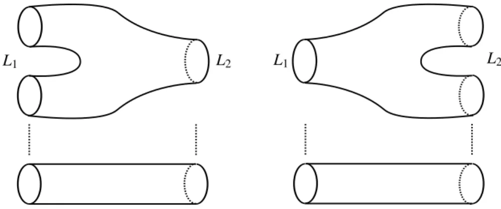
L₁ L₂ L₁ L₂

Figure 6: Merge and split cobordisms.

O-marking on the new component ofL₂. To avoid this problem we first consider the identity map in the filteredGCf theory

Id :GC(Df ₁)−→GC(Df ₂),

which clearly is a chain map since now everyO-marking is special; moreover it induces an isomorphism in homology, that preserves the Maslov grading, and a direct computation gives that it is filtered of degree 1.

Now we use Equation (9) and we get an isomorphism

Φ_Split:GH(Ld ₁)⊗W−→dGH(L₂)

that is a degree 1 filtered map which still preserves the Maslov grading. TheW factor appears because in Equation (9) we take into account the size ofDi and the number of components of

Li; while the first quantity is the same for both diagrams the linkL₂has one more component thanL₁.

iii) Merge cobordism. This cobordism (left in Figure6) represents a band move whenL₁ has one more component thanL₂. We have an isomorphism

Φ_Merge:GH(Ld ₁)−→GH(Ld ₂)⊗W.

The map is obtained in the same way as Φ_Split in the previous case, but with the difference that now it is filtered of degree 0.

L₁ L₂

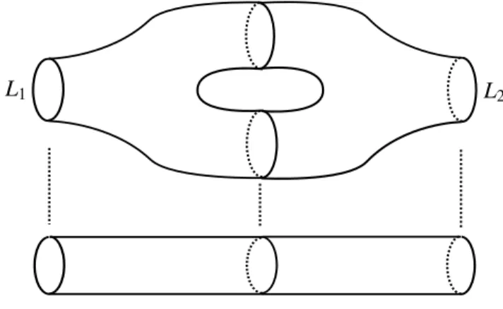
Figure 7: Torus cobordism.

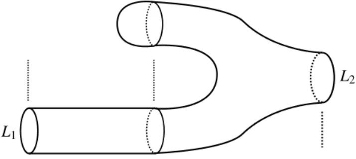
Sometimes we are more interested in when a split and a merge cobordism appear together, the second just after the first, in the shape of what we call a torus cobordism (Figure7). We have the following proposition.

L₂

L₁

Figure 8: Birth cobordism.

Proposition 4.1 Let Σ be a torus cobordism between two links L₁ and L₂. Then Σ induces a Maslov grading preserving isomorphism betweenGH(Ld ₁) anddGH(L₂), which is filtered of degree 1 .

Proof We can choose D₁ in a way that the split and the merge band moves can be performed on two disjoint bands. Then we apply twice the move shown in Figure5 and we take as map the identity. In this case the identity is a chain map becauseL₂ has the same number of components of L₁; this means that the specialO-markings inD₁andD₂ are the same and then the two differentials coincide. In this way we obtain an isomorphism in homology with Maslov grading shift and filtered degree equal to the sum of the ones in ii) and iii).

iv) Birth cobordism. A cobordism (Figure8) representing a birth move.

Since our cobordisms have boundary in both L₁ andL₂, we can always assume that a birth move is followed (possibly after some Reidemeister moves) by a merge move. Thus it is enough to define a map for the composition of these three cobordisms and this is what we do in the following proposition.

Proposition 4.2 LetΣbe a cobordism between two linksL₁ andL₂ like the one in Figure9. Then Σinduces an isomorphism Φ_BirthbetweenGH(Ld ₁) anddGH(L₂)that preserves the Maslov grading and it is filtered of degree 0.

L₂

L₁

Figure 9: A more useful birth cobordism.

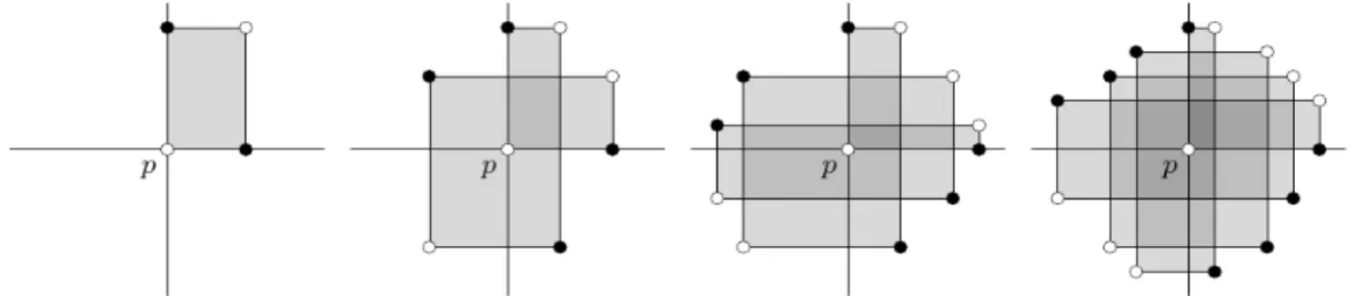
Proof The first step is to construct a maps₁ associated to the grid move shown in Figure10; note that we add a normal O-marking, since later we merge the new unknot component with an already exisiting one. Let us denote with D⁰₁ the stabilized diagram and with c =α∩β the point in the picture; then we have the inclusion i:S(D₁) → S(D⁰₁) that sends a grid state x in D₁ to the grid state in D⁰₁ constructed fromx by adding the pointc. Thens₁ :GC(Dc ₁)→ GC(Dc ⁰₁) is defined by the following formula:

s₁(x)= X

y∈S(D⁰₁)

X

H∈SL(i(x),y,c) H∩sO=∅

V₁^n1(H)·...·V_m^nm(H)y for anyx∈S(D1)

where SL(x,z,p) is the set of all the snail-like domains (the exact definition can be found in [7]

D₁

D₁ α X

β c

Figure 10: Birth move in a grid diagram.

Chapter 13) centered at p joining x to z, illustrated in Figure 11; ni(H) is the number of times H passes through O_i and m is the number of the normal O-markings of D₁. In [5] is proved that s₁ is a filtered quasi-isomorphism which induces a filtered isomorphism between GH(Ld ₁) → GHd^O(L₁t ); where the special O-markings on L₁t coincide with the ones onL₁ (the new

unknotted component has a normal O-marking). Moreover, in [14] Sarkar showed that the map s₁ is filtered of degree 0.

At this point we composes₁ with the map s₂ given by the Reidemeister moves, which is a filtered quasi-isomorphism for Theorem3.3, and finally with s₃, the identity associated to the band move of Figure5. The maps₃ induces an isomorphismGHd^O(L1t )→dGH(L2) that clearly preserves

Figure 11: Some of the snail-like domains SL(x,z,p): the coordinates of x and z are represented by the white and black circles.

the Maslov grading and again we easy compute that it is filtered of degree 0.

Hence, the composition of these three maps that we defined induces the isomorphism in the claim.

v) Death cobordism. This cobordism (Figure12) represents a death move. Since this move can also be seen as a birth move betweenL^∗₂ andL^∗₁, we take the dual map of

ΦBirth:GH(Ld ^∗₂)−→GH(Ld ^∗₁)

which exists from Proposition4.2; thenΦ^∗_Birth= Φ_Death, by Proposition3.4, is a map between dGH(L₁) anddGH(L₂). Furthermore, it is still an isomorphism that is filtered of degree 0 and preserves the Maslov grading.

L₂ L₁

Figure 12: Death cobordism.

The results for birth and death cobordisms in this section immediately give the following corollary.

Corollary 4.3 Suppose there is a birth or a death cobordism as in Figures 9and12between two linksL₁ andL₂. Then we have thatGHd(L1)∼=dGH(L2).

4.2 Strong concordance invariance

We want to prove Theorem 1.2. We remark that a strong cobordism is a cobordism Σ, between two links with the same number of components, such that every connected component of Σ is a knot cobordism between a component of the first link and one of the second link. Moreover, if the connected components of Σ are all annuli then we call Σ a strong concordance. We start by observing that Proposition4.1leads to the following corollary.

Corollary 4.4 Suppose there is a strong cobordism Σ between L₁ and L₂ such that Σ is the composition ofg(Σ)torus cobordisms, not necessarily all of them belonging to the same component ofΣ. Then Σinduces an isomorphism between dGH(L₁) and dGH(L₂), which is filtered of degree g(Σ) and preserves the Maslov grading.

Now, if we have an isomorphism F :GHd(L1) →GHd(L2) that preserves the Maslov grading and it is filtered of degree t, which means that there are inclusionsF

F^sdGH_d(L1)

⊂ F^s+tdGH_d(L2) for everyd,s∈Z, thenτ(L2)6τ(L1)+t. Hence we can prove the following theorem that immediately implies the invariance statement.

Theorem 4.5 Suppose that Σis a strong cobordism between two linksL₁ andL₂. Then

|τ(L1)−τ(L2)|6g(Σ).

Furthermore, ifL₁ andL₂ are strongly concordant thenGH(Ld ₁)∼=dGH(L₂).

Proof By Proposition B.5.1 in [7] we can suppose that, in Σ, 0-handles come before 1-handles while 2-handles come later; moreover we can say thatΣis the composition of birth, torus and death cobordisms (and obviously some identity cobordisms). Each of these induces an isomorphism in homology that also respects the Maslov grading.

For the first part, we only need to check what is the filtered degree of the isomorphism between GH(Ld ₁) and dGH(L₂), obtained by the composition of all the induced maps on each piece of Σ.

Birth, death and identity are filtered of degree 0, while, from Corollary4.4, the torus cobordisms are filtered of degreeg(Σ). Then we obtain

τ(L2)6τ(L1)+g(Σ).

For the other inequality we consider the same cobordism, but this time fromL₂ to L₁.

Now, for the second part, we observe that now there are no torus cobordisms and then the claim follows from Corollary4.3.

4.3 A lower bound for the slice genus

Suppose Σ is a cobordism (not necessarily strong) between two links L₁ and L₂. Denote with Σ₁, ...,ΣJ the connected components ofΣ. Fori=1,2 we define the integersl^k_i(Σ) as the number of components of L_i that belong to Σk minus 1; in particular l^k_i(Σ) > 0 for any k,i. Finally, we say that li(Σ) =

J

X

k=1

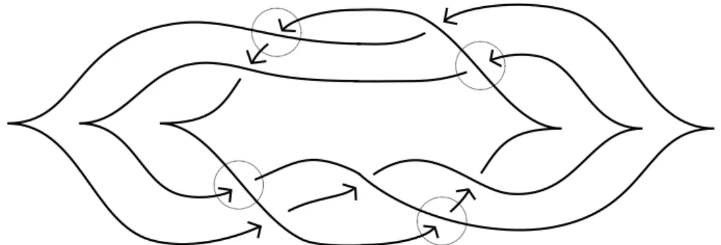
l^k_i(Σ) =ni−J, where ni is the number of component of Li. For example, if Σ is the cobordism in Figure13then J =2, ordering Σ₁ and Σ₂ from above to bottom, we have thatl₁(Σ) =3 andl₂(Σ)=4; while l¹₁(Σ)=2, l²₁(Σ)=1, l¹₂(Σ) =3 andl²₂(Σ)=1. We have the following lemma.

Lemma 4.6 If Σhas no 0,2-handles then, up to rearranging 1-handles, we can suppose that Σ is like in Figure13: there arel₁(Σ)merge cobordisms between(0,t₁),l₂(Σ)split cobordisms between (t₂,1)andg(Σ)torus cobordisms between (t₁,t₂). We have no other 1-handles except for the ones we considered before.

t₁ t₂

L₁

L₂

0 1

Figure 13

Proof We consider a connected component Σk, which is a cobordism betweenL^k₁ andL^k₂, and we fix a Morse functionf :S³×[0,1]→[0,1]. After some Reidemeister moves, by Proposition B.5.1 we can assume that all the band moves are performed on disjoint bands, in particular we can apply them in every possible order.

Since Σk has boundary in both L^k₁ and L^k₂ by the definition of cobordism given at beginning of Section4, if we take an ordering for the components of L^k₁, we can find a merge cobordism joining the first and the second component of L^k₁ at some point t in (0,1); we assume that the associated band move is the first we apply on L^k₁. Now we just do the same thing on the other components, but taking the new component instead of the first two. In this way we have that there is at₁∈(0,1) such thatΣk∩f⁻¹[0,t₁] is composed byl^k₁(Σ) merge cobordisms andΣk∩f⁻¹(t1) is a knot.

In the same way we find that, for a certain t₂ ∈(0,1), the cobordism Σk∩f⁻¹[t2,1] is composed by l^k₂(Σ) split cobordisms and Σk∩f⁻¹(t₂) is a knot.

At this pointΣk∩f⁻¹[t₁,t₂] is a knot cobordism of genus g(Σk) and from Lemma B.5.3 in [7] (see also [4]) we can rearrange the saddles to obtain a composition of g(Σk) torus cobordisms like in Figure13.

To see that there are no other 1-handles left it is enough to compute the Euler characteristic ofΣk: 2−2g(Σk)−l^k₁(Σ)−1−l^k₂(Σ)−1=χ(Σk)=−#|1-handles|.

This means that the number of 1-handles inΣk is precisely 2g(Σk)+l^k₁(Σ)+l^k₂(Σ).

From Figure13we realize that merge and split cobordisms can appear alone inΣand not always in pair like in strong cobordisms. In case ii) and iii) of Subsection4.1we see that they do not induce

isomorphisms in homology, but we find maps ΦSplit and ΦMerge that are indeed isomorphisms if restricted toGHd₀(L1)→dGH₀(L2); moreover, the filtered degree is 1 for split cobordisms and 0 for merge cobordisms. Since we are looking for informations onτ, this is enough for our goal and then we can prove the following inequality.

Proposition 4.7 Suppose Σis a cobordism between two links L₁ andL₂. Then

|τ(L1)−τ(L2)|6g(Σ)+max{l₁(Σ),l₂(Σ)}.

Proof By Theorem4.5, we can suppose that there are no 0 and no 2-handles in Σ. We can also assume thatΣis like in Lemma4.6.

All of these cobordisms induce isomorphisms of the homology in Maslov grading 0. The number of torus cobordisms isg(Σ) while the number of split cobordisms (that are not part of torus cobordisms) isl₂(Σ). This means that

τ(L2)6τ(L1)+g(Σ)+l₂(Σ).

Now we do the same, but considering the cobordism going from L₂ toL₁, as we did in the proof of Theorem4.5. We obtain that

τ(L₁)6τ(L₂)+g(Σ)+l₁(Σ).

Putting the two inequalities together proves the relation in the statement of the theorem.

IfL is ann-component link, from Proposition4.7we have immediately Equation (1):

|τ(L)|+1−n6g₄(L)

which, as we already said, is a lower bound for the slice genus of our link. Indeed, we can say more by using Equation (10) and observing that g₄(L^∗)=g₄(L):

max{|τ(L)|,|τ^∗(L)|}+1−n6g₄(L).

5 The GH

version of filtered grid homology

5.1 A different point of view

The collapsed filtered complex cGC⁻(D) for a grid diagram D is the free F[V1, ...,V_grd(D)−n,V]- module generated by the set of grid states S(D). This ring has one more variableV, compared to the ring we considered for GC(D), associated to the specialc O-markings. The differential ∂⁻ is defined as following:

∂⁻x= X

y∈S(D)

X

r∈Rect^◦(x,y)

V₁^O1(r)·...·V_m^Om(r)·V^O(r)y for anyx∈S(D) wherem=grd(D)−n andO(r) is the number of specialO-markings in r.

It is clear from the definition that

GC(D),c ∂b

= cGC⁻(D), ∂⁻ V =0 .

The collapsed filtered unblocked homology cGH⁻(L) is the homology of our new complex and it is a link invariant; but now each levelF^scGH⁻(L) has also a structure of anF[U]-module given by U[p]=[Vip]=[Vp] for every i=1, ...,mand [p]∈cGH⁻(L). The groupsF^scGH⁻_d(L) are still finite dimensional over Fand so we can define the functionN as

N_L(d,s)=dim_F F^scGH⁻_d(L) F^s−1cGH⁻_d(L).

We expect the functionN to be a strong concordance invariant, possibly better thanT. We can compute the function N of the unknot:

N(d,s)=

(1 if (d,s)=(2t,t), t60

0 otherwise

and we know that

cGH⁻(L)∼=_F[U]cGH⁻(_n)∼=_F[U]F[U]²ⁿ⁻¹ as anF[U]-module, where n is the number of component ofL.

Since dim_FcGH⁻₀(L) is still equal to 1, we can define an invariantν exactly like we did in Subsection 3.1for τ. A version of the ν-invariant has been introduced first by Jacob Rasmussen in [12] and he proved that it is a concordance invariant for knots. In [3] Hom and Wu found knots whose ν-invariant gives better lower bound for the slice genus thanτ.

Since H∗,∗ gr cGC⁻(D)

is isomorphic to the homology cGH⁻(L) of [7] and NL(0, ν(L)) = 1 for every diagram DofL, we have that cGH_0,ν(L)⁻ (L) is non-trivial. Hence, if the homology group cGH₀⁻(L) is non-zero only for one Alexander gradings, we can argue thatν(L)=s. This method can be used to compute theν-invariant of some links.

We can also define the (uncollapsed) filtered unblocked homology as the homology of the complex GC⁻(D), ∂⁻

, whereGC⁻(D) is the freeF[V1, ...,V_{grd (D)}]-module over the grid states ofD; there are no specialO-markings this time.

We see immediately that for everyn-component linkLis GH⁻(L)∼=F[U₁, ...,Un]

with generator in Maslov grading 0, but the filtration will of course depend on L.

5.2 Proof of Theorem1.3

We use the complexcGC⁻to prove that, for everyn-component linkL, an integersgivesT_d,s(L)6=0 for some d if and only if s belongs to the τ-set of L. To do this, given C a freely and finitely generated F[U]-complex, we define two set of integers: τ(C) and t(C). First we call B_τ(C) a homogeneous, free generating set of the torsion-free quotient of H∗,∗(gr(C)) as an F[U]-module;

thenτ(C) is the set ofs∈Zsuch that there is a [p]∈ B_τ(C) with bigrading (d,−s) for somed∈Z.

Similarly,t(C) is the set of the integers ssuch that the inclusion i_s:F^s−1H_∗

C U=0

,−→ F^sH_∗ C

U=0

is not surjective. Note that the setB_τ(C) is not unique, butτ(C) and t(C) are well-defined.

We say that s ∈ τ(C) has multiplicity k if there are k distinct elements in B_τ(C) with bigrading (∗,−s), while a number u ∈ t(C) has multiplicity k if Cokeri_u has dimension k as an F-vector space.

Clearly, ifDis a grid diagram ofL,t cGC⁻(D)

is the set of the values ofswhere the functionTLis supported; moreover, we already remarked thatH_∗,∗ gr cGC⁻(D)

is isomorphic tocGH⁻(L) and thenτ cGC⁻(D)

is theτ-set ofL. Hence our goal is to prove thatt cGC⁻(D)

=τ cGC⁻(D) , generalizing Proposition 14.1.2 in [7].

Consider the complex

C= cGC⁻(D) V₁=...=Vm=U ,

wherem=grd(D)−nandU is the variable associated to the specialO-markings. Then we define C as the complexCJ1−n−m,−mK.

We introduce a new complexC⁰ =C ⊗_F[U]F[U,U⁻¹] and we define aZ⊕Z-filtration onC⁰ in the following way: F^x,∗C⁰ =U^−xC for every x∈Z, F^∗,yC⁰ =F^yC⁰ ={p∈ C⁰|A(p)6y} for every y∈ZandF^x,yC⁰ =F^x,∗C⁰∩ F^∗,yC⁰ =U^−xF^y−xCfor everyx,y∈Z. The first step is to prove that τ(C)=t(C).

We have that

C U=0

∼=GC(D)f ∼= F^0,∗C⁰ F^−1,∗C⁰ ; moreover, for every integers we claim that

F^sGC(D)f ∼= F^0,sC⁰ F^−1,sC⁰ .

Since, from Lemma 14.1.9 in [7], it isF^x,yC⁰ ∼=F^y,xC⁰ for everyx,y∈Z, then we have that

(13) F^s C

U=0

∼=F^sGC(D)f J1−n−m,−mK

∼= F^s,0C⁰ F^s,−1C⁰ .

Using this identification we obtain thatt(C) coincides with set ofs∈Zsuch that the map

(14) H_∗

F^s−1,0C⁰ F^s−1,−1C⁰

,−→H_∗

F^s,0C⁰ F^s,−1C⁰

is not surjective.

Now we consider the complex gr(C), which is equal to M

t∈Z

F^0,tC⁰

F^0,t−1C⁰. We have that the map U^t : F^0,tC⁰

F^0,t−1C⁰ −→ F^−t,0C⁰ F^−t,−1C⁰ is an isomorphism and F^−t,0C⁰

F^−t,−1C⁰ is a subspace of F^∗,0C⁰

F^∗,−1C⁰ for every integer t. From Lemma 14.1.12 in [7] the latter filtered complex is isomorphic to gr(C)

U=1, but it is also isomorphic to GC(D)f J1−n−m,−mKfor Equation (13). In this way we can define a surjective map

Ψ: gr(C)−→ gr(C) U=1

and it is easy to see that Ψ(B_τ(C)) is still a homogeneous, free generating set of the homology;

furthermore, if [p] is a torsion element in H_∗,∗(gr(C)) then [Ψ(p)] =[0]. This means that τ(C) is the set of−t∈Zsuch that the map

(15) H∗

F^−t−1,0C⁰ F^{−t−1,−1}C⁰

,−→H∗

F^−t,0C⁰ F^−t,−1C⁰

is not surjective.

If we change −twith s in Equation (15) then we immediately see that it coincides with Equation (14) and soτ(C)=t(C). Moreover, we can say that an integer inτ(C) has multiplicitykif and only if it has multiplicity k int(C). Finally, since the map U^t drops the Maslov grading by 2t, we have that if there is a [p]∈ B_τ(C) with bigrading (d,s) then there is a generator ofgGH(D)J1−n−m,−mK with grading and minimal level (d−2s,−s).

The second and final step is to show that the previous claim impliest cGC⁻(D)

=τ cGC⁻(D) . From Lemma 14.1.11 in [7] we have the filtered quasi-isomorphisms C ∼=cGC⁻(D)⊗W^⊗m and C ∼=cGC⁻(D)⊗(W^∗)^⊗m, whereWis the two dimensionalF-vector space with generators in grading and minimal level (d,s) = (0,0) and (d,s) = (−1,−1). Thus t cGC⁻(D)

and τ cGC⁻(D) completely determine τ(C) and t(C), so this means that they coincide and the proof is complete.

Obviously, the conclusions about multiplicities and Maslov shifts are still true.

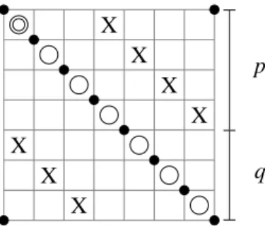
From [7] Chapter 8 we know that there is only one element [p] ∈ B_τ cGC⁻(D)

with bigrading (−2τ₁,−τ₁) and only another one [q] with bigrading (−2τ₂+1−n,−τ₂). Then the proof of Theorem1.3implies that there are two non-zero elements in dGH(L) in grading and minimal level (0, τ₁) and (1−n, τ₂). Since, from the definition ofτ andτ^∗, we also know that there are only two generators ofGH(L) in Maslov grading 0 and 1d −n; we have the following corollary.

Corollary 5.1 Take a grid diagramDof ann-component linkLand consider a setB_τ cGC⁻(D) . If [p],[q] ∈ B_τ cGC⁻(D)

are such that [p] is in bigrading (−2τ₁,−τ₁) and [q] is in bigrading (−2τ₂+1−n,−τ₂) then τ(L)=τ1 andτ^∗(L)=τ2.

6 Applications

6.1 Computation for some specific links

In general it is hard to say when a sum of grid states is a generator of the homology, but the following lemma provides an example where we have useful information.

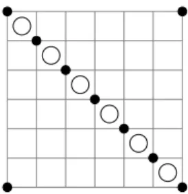
Lemma 6.1 Suppose L is an n-component link with grid diagram D and x ∈ S(D) as in Figure 14. Then[x] is always the generator ofdGH₀(L) andcGH⁻₀(L). Furthermore, τ(L)=ν(L)=A(x). Proof We show that M(x) = 0, ∂xb = ∂⁻x = 0 and that for every other grid state y of D it is M(y)60.

i) The fact thatM(x)=0 is trivial.

ii) For every y ∈S(D) there are always 2 rectangles in Rect^◦(x,y) and they contain no O, so they cancel when we compute the differential.