Entanglement detection and quantum metrology in quantum optical systems

(1)

Entanglement detection and quantum metrology in quantum optical systems

(Összefonódottság észlelése és kvantummetrológia kvantumoptikai rendszerekben)

Doctoral Dissertation

submitted to the Hungarian Academy of Sciences

Géza Tóth

Wigner Research Centre for Physics

Budapest

2019

(2)

(3)

Chapter 1 Introduction

Although the most important principles of quantum mechanics were laid down by Schrö- dinger, Neumann and their contemporaries by the 1930’s, a novel development started in the 1980’s with applying information theoretical concepts to quantum mechanics. The new interdisciplinary field, Quantum Information Theory (QIT), is concerned with fundamental issues such as entanglement, non-locality, as well as applications. The notion of entanglement was introduced by Schrödinger in 1935. In spite of its long past, several questions remain unanswered. Only quite recently, significant progress has been achieved in understanding entanglement [1, 2].

Entanglement appears in most of the sub-fields of QIT, for example in quantum computation. Quantum computers can outperform classical ones in certain tasks, such as prime factoring and searching, since they exploit superposition and entanglement [3, 4].

Quantum teleportation can be used to move the state of a particle to a distant particle [5]. For quantum cryptography, one can use entangled particles to provide secure communication between two parties. In all these cases, successful experiments have already been carried out while quantum cryptography is perhaps not far from becoming a real life application. Moreover, entangled quantum states are shown to outperform non-entangled ones in certain metrological application and might lead to more exact atomic clocks [6, 7].

Entanglement also appears as a natural goal in today’s quantum experiments (e.g., [8–

12]). In this way, quantum information science, and in particular entanglement theory, can play a crucial role in the technological development of quantum control and quantum engineering. Finally, the realization of larger and larger entangled quantum systems might also help to answer fundamental questions concerning quantum theory, such as the appearance of a classical macroscopic world based on a quantum microworld (e.g., [13]).

Next, we will first review quantum systems that make it possible to create many- particle entanglement. Then, we present short reviews of entanglement theory and quan-

(8)

CHAPTER 1. INTRODUCTION 2 tum metrology. Finally, we outline the theory of Bell inequalities.

1.1 Interesting quantum states

In this section, we present some quantum states relevant for quantum information. This will help us to have an idea about the recent quantum experiments preparing highly entangled quantum states.

A pure product state of anN-particle system can be given as

|Ψ₁i ⊗ |Ψ₂i ⊗...⊗ |Ψ_Ni, (1.1.1) where |Ψ_ni is the state of the nth particle. If the system is in such a state, then there are no correlations between the particles, that is, hA_nB_mi=hA_nihB_mi for anyA_n and B_m operators measured on particle n and m, respectively.

For quantum information applications, we need highly correlated quantum states. One of such states is thesinglet state given as

√1

2(|01i − |10i). (1.1.2)

The singlet state is often called maximally entangled among two-qubit states, where

“qubit” means a two-state system.

Highly entangled states are studied also in multiparticle systems. One of the most interesting states is the Greenberger-Horne-Zeilinger (GHZ) state [14], which is just a superposition of a state in which all particles are in state “0” and another one in which all particles are in state “1”

|GHZ_Ni= 1

√2

|00..0i

| {z }

+|11..1i

N qubits

, (1.1.3)

where N is the number of two-state particles. In a sense, one can call this state a Schrödinger cat state.

GHZ states are in the symmetric subspace. They are very fragile to noise, since even after a single particle is lost, we obtain a trivial mixture of two product states. There are symmetric entangled states that are more robust to noise. One of them is calledW-state,

(9)

CHAPTER 1. INTRODUCTION 3 and is defined as

√1

2(|100..00i+|010..00i+...+|000..01i). (1.1.4) It is just a superposition of all permutations of the states in which a single particle is in state “1” and all the others are in state “0” .

States with more than 1 excitations are also studied intensively. AnN-qubit symmetric Dicke state with m excitations is defined as [15, 16]

|m, Ni:=

N m

−¹₂

X

k

P_k(|1₁,1₂, ...,1_m,0_m+1, ...,0_Ni), (1.1.5) where {P_k} is the set of all distinct permutations of the spins. |1, Ni is the N-qubit W state given in Eq. (1.1.4). In the literature and also in this thesis, for an even N, Dicke state often means just the state|N/2, Ni, since it is the most studied state and the most entangled one among the states (1.1.5).

Finally, quite recently another family of quantum states, called cluster states, have raised considerable interest. While the multiparticle states mentioned so far were symmetric, the cluster state is a state in a one-dimensional spin chain. It can be given explicitly with an Ising dynamics starting from a product state as

|C_Ni=U_C |00..0i_x

| {z } , N qubits

(1.1.6)

wherexindicates that the state is given in thex-basis, the unitary evolution is defined as UC = exp(−iHC

π

4), (1.1.7)

and the Hamiltonian is

HC =

N−1

X

n=1

(1−σ⁽ⁿ⁾_z )(1−σ⁽ⁿ⁺¹⁾_z ), (1.1.8) where σ⁽ⁿ⁾_l for l = x, y, z denotes Pauli spin matrices in the thesis¹. Note that U_C² = 1. Hence, applying U_C again we arrive at the initial product state. Cluster states are interesting, since they can be used for a quantum computation scheme which is not based on a unitary evolution, but on single-particle measurements. With two-dimensional cluster states, even universal quantum computation can be realized. In the literature, it is called measurement-based quantum computing [17].

1We also use theX⁽ⁿ⁾, Y⁽ⁿ⁾, Z⁽ⁿ⁾ notation in some part of the thesis, following the literature.

(10)

CHAPTER 1. INTRODUCTION 4

1.2 Physical systems

In this section, we will discuss some quantum optical systems, in which entanglement has been created.

(i) Systems in which the particles are addressable, with typically 5-10 particles Photons are one of the most versatile systems for quantum experiments. They encode the “0” and “1” in the horizontal and vertical polarization of the photons, respectively.

While photons do not interact with each other, parametric down-conversion and selective detection makes it possible to obtain a large variety of quantum states. Photonic setups can typically create a single quantum state, or a family of states. If we would like to obtain another state, we need to build another experimental setup. However, the quantum state that we are aiming to create can be obtained with a large fidelity. Using more than one degrees of freedom for a single photon, even a ten-qubit GHZ state has been created [18].

Since a photon can take more than two degrees of freedom, a rapid increase is expected above 10qubits [19].

Trapped ions are another possibility to create multi-particle quantum states. Ions do not interact directly, only through phonons. Thus two-qubit gates must be realized through involving the vibrational states of the chain of ions. Applying different pulse sequences can be used, in principle, to realize various entangled states with the same ion trap. In practice, there are states that are more suitable for the realization in an ion trap than other states. Ion traps have a limit of around 10−20 atoms, hence they are now aiming to combine several such traps to increase to number of ions further. An eight-qubit W-state has been realized with ion traps [20], as well as GHZ states up to 14qubits [21].

(ii) Systems in which only collective quantities can be measured, with typically 10⁶−10¹² particles

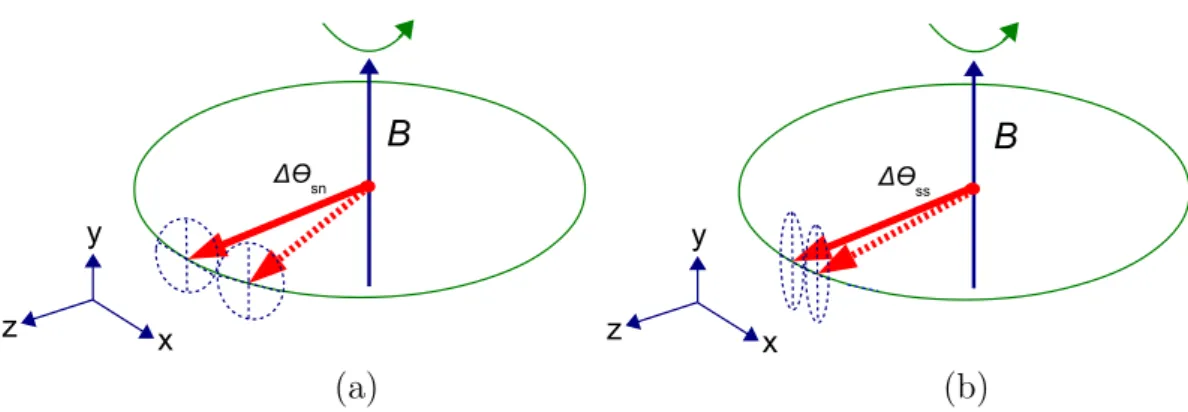
In experiments with cold atomic ensembles, the quantum information is stored in the internal states of the atoms. The atoms are in a vacuum chamber and do not interact with each other [22]. However, by shining light through the chamber and subsequently detecting it, it is possible to entangle the atoms. This way, it is also possible to decrease the variances of collective spin observables to a considerable extent, which is called spin squeezing [23]. Quantum states obtained this way become useful for quantum metrology, as shown in Fig. 1.1. That is, they can provide a better accuracy in measurements than a state in which the spins are not correlated. In such systems, continuous variable quantum teleportation was realized [24], two large ensembles were entangled with each other [10], and a quantum memory for light was realized [25]. The optical depth can be enhanced much further if the ensemble is placed inside an optical cavity. With that technique, very

(11)

x y z

B

Δϴsn

x y z

B

Δϴ_ss

(a) (b)

Figure 1.1: (a) Magnetometry with an ensemble of spins. All spins point into thez direction. (Solid arrow) The large collective spin precesses around the magnetic field pointing into they direction. (Dashed arrow) After a precession of an angle ∆θ_sn,the uncertainty ellipse of the spin is not overlapping with the uncertainty ellipse of the spin at the starting position. Hence,∆θ_sn is close to the uncertainty of the phase estimation, which coincides with the shot-noise limit, indicated by the subscript “sn.” (b) Magnetometry with an ensemble of spins. All spins point to the z direction and are spin squeezed along the x direction. The uncertainty of the phase estimation is close to the angle ∆θ_ss, which is smaller than ∆θ_sn due to spin squeezing, indicated by the subscript “ss.”

recently, they achieved a 100 times squeezing in such systems [26].

Bose-Einstein condensates can also be used to create correlated states of an ensemble of two-state atoms. The quantum information is stored again in the internal states of the atoms. However, now the atoms interact with each other which can be used to create spin squeezed states [7, 27–29] and Dicke states [30, 31]. Clearly, a bosonic particle has an integer spin. Often, they use particles with a spin j = 1, hence such a particle has three states corresponding to the three eigenvectors of the spin componentj_z.Often, the experimenters would like to work with two-state atoms. Then, the two-state subsystems are created artificially, such that they keep one of the three levels, typically the j_z = 0 level, unpopulated. There are also experiments aiming to realize quantum states with particles with more than two internal states (e.g., Ref. [11]). The advantage of such experiments is that the two-state subsystems need not be created artificially.

Bosonic atoms can also be placed in a lattice. In a paradigmatic experiment they filled around 100 000 cold atoms in a 3D optical lattice [32]. The quantum information was again stored in the internal states of the atoms. Atoms with different states were trapped with different trapping potentials. Moving one of these potentials relative to the other one, they could achieve that atoms get delocalized and interact with atoms at different lattice sites. They used these techniques to realize a 2D array of Ising spin chains and create large scale entanglement [33]. We note that nowadays in some optical lattice experiments they even have access to individual lattice sites [34].

(12)

1.3 Entanglement detection

In this section we will discuss, how to interpret the results of various experiments aiming at creating highly entangled quantum states. A review can be found in Ref. [2].

When a quantum state is created, we can obtain lots of data about the state. However, we must be able to characterize the success of the experiment with few data. For example, one can measure the fidelity of the state with respect to the state we intended to create.

This is a number between 0 and 1. If the fidelity is large, then the experiment was successful. Another possibility is to prove that the quantum state is entangled. This, as we later discuss, tells us that the state is qualitatively different from non-entangled or separable states.

The theory of entanglement started with the seminal paper of R. F. Werner in 1989 [35], that defined entangled states as they are defined now. Next, we summarize some important aspects of entanglement theory. Let us imagine for a moment, that we have only pure quantum states in nature. In this case, it would be sufficient to talk aboutpure product states and pure entangled states. The pure product states are also called pure separable states. This classification is considered in condensed matter, when they talk about the properties of ground states of certain spin chain Hamiltonians. In this case, product states have the property that they do not exhibit any correlation between the particles.

In the real word, we cannot prepare pure states in an experiment. We can only aim at preparing a pure state, but the result will be a mixed state. (We have to remember that when a quantum state is prepared, we always have to talk about a series of experiments, not only a single one.) Thus, we have to generalize the notion of pure separable states to mixed separable states. A mixed separable state is just a mixture of pure product states.

Any state that is not separable is called anentangled state.

Since separable states are just mixtures of trivial product states, quantum interaction is not needed to produce them. This does not exclude the possibility that such an interaction was present. However, we cannot prove it based on the density matrix. In the case of entangled density matrices, we can know that quantum interaction provably contributed to the creation of the state.

Note that separability does not exclude the possibility that the measurements find correlations in separable states, which is not possible for pure product states. However, these correlations can be achieved by operations acting locally on the subsystems, and classical communication among the subsystems, which is the quantum information theoretical analogue of classical interaction. Such operations are called local operations and classical communication (LOCC), see Sec. 2.1.2.

(13)

CHAPTER 1. INTRODUCTION 7 Since entanglement is an important property of the quantum state, there has been a large effort to decide whether a quantum state is entangled. In short, we have to decide whether the density matrix of a two-particle or multi-particle quantum state can be written as a mixture of product states. It turns out that this problem is not solvable in general [36]. There are only necessary conditions for separability. If they are violated, then we know that the state is entangled. However, we do not detect all entangled states this way.

After a general review on entanglement theory, let us discuss how entanglement can be detected in various systems. First, we consider few particle states, corresponding to systems of type (i) of Sec. 1.2. After a multi-particle quantum state is created, one can try to obtain the density matrix of the quantum state by quantum state tomography. This is possible only for small systems (i.e., 10-20 two-state particles), since the number of degrees of freedom (i.e., the number of independent real parameters) increases exponentially with the number of particles. There are also other methods that do not recover the full density matrix, only a part of it, such as permutationally invariant tomography (Sec. 6). They can be used for larger systems.

One of the necessary conditions for separability is the criterion based on the positivity of the partial transpose (PPT). It is based on transposing a density matrix of a two-particle system according to one of the subsystems. Simple algebra shows that the matrix obtained is positive-semidefinite for all separable states. Hence, if the result of the transformation above is not positive-semidefinite, then the state was entangled. This way, we can detect all entangled states in 2×2 and 2×3systems (i.e., composite systems consisting of two two-state systems, and a two-state system and a three-state system, respectively). There are other criteria, such as the Computable Cross Norm-Realignment Criterion (CCNR), that detects some entangled states that are not detected by the PPT criterion. However, the CCNR criterion is in general not stronger than the PPT criterion.

So far we discussed entanglement detection in the case that the density matrix is fully known. As we mentioned, this can happen only for small systems. Moreover, even for small systems typically it is not possible to measure all the correlations needed to obtain the density matrix. Fortunately, it is possible to detect entanglement by measuring only a single operator. Such an operator is called anentanglement witnes. Clearly, entanglement witneses detect only some entangled states. However, the infinitely many entanglement witnesses altogether detect all entangled states.

There is a large literature on how to design entanglement witnesses. There are witnesses which detect entanglement close to Greenberger-Horne-Zeilinger states [37–39], cluster states [39–41], and Dicke states [42–46]. A multi-particle quantum operator cannot typically be measured directly. It must be decomposed into the sum of product

(14)

CHAPTER 1. INTRODUCTION 8 operators. When looking for entanglement witnesses, it is important to look for ones that can be decomposed into the sum of few terms, hence they are easy to measure.

So far, we considered quantum systems of few particles. Next, we discuss entanglement detection in the many-particle ensembles corresponding to systems of type (ii) of Sec. 1.2.

On the one hand, in large systems it is impossible to obtain the density matrix due to the very large number of degrees of freedom. On the other hand, typically the particles are not individually addressable and there are few means that can be used to manipulate them, both for creating highly entangled quantum states or to verify their entanglement content.

In a system of many particles, typically one can measure the expectation values of collective quantities, such as the collective angular momentum components. We can also measure the variance of these quantities. These are already sufficient to detect entanglement in an ensemble of many, say 10³ or10¹², particles. The most known entanglement criterion of this type is the spin-squeezing inequality. Later, the full set of such conditions have been determined for spin-1/2 particles [47]. That is, we cannot find further conditions that detect more states based on the expectation values and variances of collective angular momentum components. Spin squeezing conditions can detect not only entanglement, but can obtain a lower bound on the entanglement depth. In other words, apart from telling “entangled”, they can also say, how many particles are entangled with each other.

1.4 Quantum metrology

Apart from detecting entanglement, it is also desirable to prove that the quantum state is useful for some application. One of the most important applications is quantum metrology [48–54]. Indeed, spin-squeezed states mentioned above can be used for quantum metrology and they provide a better precision in magnetometry than non-entangled states [23].

The central notion of the field is the quantum Fisher information. It determines the best achievable precision in linear interferometers for a given quantum state. The larger the quantum Fisher information, the better the precision.

Recently, it has even been proven that entanglement is needed to reach the maxi- mal quantum Fisher information and hence, the best precision in metrology [52, 55, 56].

Hence, proving metrological usefulness can also be used for entanglement detection. In more details, higher and higher values of the quantum Fisher information in linear interferometers can be achieved only by quantum states with a larger and larger entanglement depth. This makes it possible to detect the entanglement depth by measuring precision

(15)

CHAPTER 1. INTRODUCTION 9 in some interferometric task carried out with the quantum state.

1.5 Bell inequalities

In this section, we briefly describe the theoretical development leading later to mod- ern entanglement theory. First of all, we have to mention the seminal paper about the Einstein-Podolsky-Rosen (EPR) paradox published in 1935 [57]. It studied quantum measurements on a two-particle singlet, when the particles are far away from each other. It pointed out several effects unusual from the point of view of classical physics, which they called “spooky action at a distance”.

Based on these ideas, Bell developed his famous inequalities in 1964 [58], which were followed by other similar relations [59]. In general, Bell inequalities are inequalities that are constructed for bipartite or multipartite systems. They are inequalities with correlations terms that are fulfilled by all so-called local hidden variable (LHV) models (Sec. 9.1.2), which assume that the results of a quantum measurement exist before the measurement. There are quantum states, such as the trivial product states, that do not violate any Bell inequality. They noticed that pure states violating Bell inequalities are often highly correlated.

In Ref. [35], entangled states have been shown that do not violate any Bell inequality.

It has been conjectured by A. Peres in 1999, that bound entangled states, i.e., entangled states with a positive partial transpose mentioned before, does not violate a Bell inequality [60]. The conjecture is reasonable since bound entangled states possess a weak form of entanglement. After a long search for counterexamples, the conjecture has been proven to be false in 2014 since some bound entangled states have been found that violate a Bell inequality [61].

On the other hand, all states violating a Bell inequality are entangled. Hence, Bell inequalities can be used for entanglement detection, even if entanglement theory did not exist when they were created. There are also other connections to entanglement theory.

Bell inequalities, like entanglement witnesses, are typically also designed for specific quantum states. There are Bell inequalities that detect states close to two-spin singlets [62], GHZ states [63], or cluster states [64–66].

1.6 Structure of the thesis

Next, we will present the topics considered in this thesis, mentioning also the relevant publications. First of all, we would draw the attention to the review articles on quantum

(16)

CHAPTER 1. INTRODUCTION 10 entanglement theory [2] and quantum metrology [52].

The thesis is organized as follows. At the beginning of each Chapter, we give a short reference to relevant publications belonging to thesis. In each Chapter, we present some sections explaining the background. Then, sections with our own results follow.

In Chapter 2, we discuss entanglement detection with few correlation terms. In particular, we will consider entanglement detection with spin chain Hamiltonians [67, 68].

In Chapter 3, we consider detection of multipartite entanglement close to graph states, which also include cluster states and GHZ states [39, 41, 69]. We also discuss how to estimate the fidelity with respect to such states [39, 41]. An experimental application of this scheme is described in Ref. [40]. In Chapter 4, entanglement detection close to Dicke states is discussed [42]. We will also show how to measure the entanglement conditions ef- ficiently [46]. We also show examples of entanglement conditions that need only collective measurements [42]. The experimental applications of this scheme are in Ref. [43, 44]. In Chapter 5, the relation between entanglement and permutational symmetry is discussed.

We will present symmetric states that are not detected by the PPT criterion [70]. In Chapter 6, we discuss an efficient tomographic method for permutationally invariant systems [71]. Its advantage is that the number of measurements needed scales quadratically with the number of qubits. This makes it possible to carry out tomography of large systems. In Chapter 7, entanglement detection with collective observables are discussed.

A generalized spin sqeeezing entanglement condition is presented that detects entanglement close to singlet states [69]. Later, a complete set of entanglement criteria based on collective observables is presented [47, 72]. In Chapter 8, the relation of multipartite entanglement and quantum metrology is discussed. We show that full multipartite entanglement is needed to reach the maximum sensitivity [56]. In Chapter 9, Bell inequalities for graph states are presented [66].

(17)

Chapter 2 Entanglement detection with correlations

In this Chapter, we will consider entanglement detection with spin chain Hamiltonians, described in Refs. [67, 68].

2.1 Background

2.1.1 Entanglement

What kind of quantum states should experiments aim at creating? Let us consider first pure states. Clearly, product states of the type

|Ψ⁽¹⁾i ⊗ |Ψ⁽²⁾i ⊗...|Ψ^(N)i (2.1.1) are not that interesting. Such states can be created without any interaction between the parties. On the other hand, pure multipartite quantum states that are not product states have to be created via an interaction between the parties.

Let us turn now to mixed states. A quantum mixed state is (fully) separable if it can be written as [35]

%sep=X

m

pmρ⁽¹⁾_m ⊗ρ⁽²⁾_m ⊗...⊗ρ^(N)_m , (2.1.2) whereρ⁽ⁿ⁾m are single-particle pure states and N is the number of the particles. Separable states are essentially states that can be created without an inter-particle interaction, just by mixing product states. States that are not separable are called entangled.

(18)

CHAPTER 2. ENTANGLEMENT DETECTION WITH CORRELATIONS 12 Entangled states are more useful than separable ones for several quantum information processing tasks, such as quantum teleportation, quantum cryptography, and, as we will show later, for quantum metrology [1, 2]. Entanglement is connected to older notions of quantum physics, such as Bell inequalities, as we have mentioned in Sec. 1.5.

Entanglement is also related to non-classicality, a central concept in quantum optics [73].

2.1.2 Local Operations and Classical Communication

Local Operations and Classical Communication (LOCC) are some series of the following operations.

• Local unitaries, i.e., unitaries of the type

U⁽¹⁾⊗U⁽²⁾⊗...⊗U^(N), (2.1.3) where U⁽ⁿ⁾ acts onn^th party of the N-partite state.

• Local von Neumann measurements and local generalized measurements, i.e., local positive-operator valued measures (POVM).

• Local unitaries or measurements conditioned on measurement outcomes on the other party.

Such operations cannot produce an entangled state from a separable one given in Eq. (2.1.2) [1, 2]. Note, however, that such operations can create correlations starting from a product state.

2.1.3 Multipartite entanglement and entanglement depth

In the many-particle case, it is not sufficient to distinguish only two qualitatively different cases of separable and entangled states. For example, an N-particle state is entangled, even if only two of the particles are entangled, as in the state

|Ψi= 1

√2(|00i+|11i)⊗ |0i^⊗(N−2). (2.1.4) Usually, we would not call the state given in Eq.(2.1.4) multipartite entangled. On the other hand, there are quantum states in which all theN particles are entangled with each other. One of the most important such highly entangled states is the GHZ state defined in Eq. (1.1.3). Hence, the notion of genuine multipartite entanglement [37, 38] has been

(19)

CHAPTER 2. ENTANGLEMENT DETECTION WITH CORRELATIONS 13 introduced to distinguish partial entanglement from the case when all the particles are entangled with each other. It is defined as follows. A pure state is biseparable, if it can be written as a tensor product of two multi-partite states

|Ψi=|Ψ₁i ⊗ |Ψ₂i. (2.1.5) A mixed state is biseparable if it can be written as a mixture of biseparable pure states.

A state that is not biseparable is genuine multipartite entangled. Genuine multipartite entanglement is one of the notions most used in nowadays experiments with ions and photons [18, 19, 21, 38, 43–45, 74–77]. A quantum system possessing entanglement of this type cannot be obtained from entangled systems of smaller size by trivial operations, without real quantum interaction. For example, by merely adding a particle to a system with N-qubit genuine multipartite entanglement, without interaction, it is not possible to get a state with (N + 1)-qubit genuine multipartite entanglement. This way, if in an experiment genuine multipartite entanglement of (N + 1) qubits is detected, then this experiment provides something qualitatively new compared toN-particle experiments.

In the many-particle scenario, further levels of multi-partite entanglement must be introduced since verifying full N-particle entanglement for N = 1000 or 10⁶ particles is not realistic. In order to characterise the different levels of multipartite entanglement, we start first with pure states. We call a state k-producible, if it can be written as a tensor product of the form

|Ψi=⊗_m|ψ_mi, (2.1.6)

where |ψ_mi are multiparticle states with k_m ≤ k particles. A k-producible state can be created in such a way that only particles within groups containing not more than k particles were interacting with each other. This notion can be extended to mixed states by calling a mixed statek-producible if it can be written as a mixture of purek-producible states. A state that is not k-producible contains at least (k + 1)-particle entanglement [78, 79]. Using another terminology, we can also say that the entanglement depth of the quantum state is larger than k [23]. An N-qubit state with an entanglement depth N is genuine multipartite entangled.

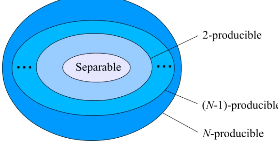
It is instructive to depict states with various forms of multipartite entanglement in set diagrams as shown in Fig. 2.1. Separable states are a convex set since if we mix two separable states, we can obtain only a separable state. Similarly, k-producible states also form a convex set. In general, the set ofk-producible states contains the set ofl-producible states if k > l.

An even more detailed classification of multipartite entangled states is possible, into which thek-producibility based classification fits naturally. It is called partial separability

(20)

CHAPTER 2. ENTANGLEMENT DETECTION WITH CORRELATIONS 14

Separable

2-producible

(N-1)-producible N-producible

... ...

Figure 2.1: Sets of states with various forms of multipartite entanglement. k-producible states form larger and larger convex sets. 1-producible states are equal to the set of separable states. The set of physical quantum states is equal to the set of N-producible states.

classification [80, 81], and it takes into account all the possible ways how the states can be mixed by the use of pure states separable with respect to different splits.

2.1.4 Entanglement witnesses

An observable W is entanglement witness if it fulfils the following two requirements [82, 83]:

(i) hWi ≥0 for all separable states, (ii) hWi<0for some entangled state.

In another context, entanglement witnesses are entanglement criteria that are linear in operator expectation values.

Entanglement witnesses can also be designed such that they detect no entanglement in general, but a certain type of entanglement, i.e., only genuine multipartite entanglement.

2.1.5 Robustness to noise for entanglement witnesses

There are infinite number of entanglement witnesses that can be used to detect a given quantum state as entangled. We have to choose one of them, by evaluating the witnesses based on their usefulness. One of the most important requirements is that the witness

(21)

CHAPTER 2. ENTANGLEMENT DETECTION WITH CORRELATIONS 15 should have a large robustness to noise. In an experiment that aims to prepare a pure state

|Ψi,the result is, of course, a mixed state, which can typically be very well approximated by the original pure state mixed with white noise as

%(p_noise) = (1−p_noise)|ΨihΨ|+p_noise%_cm, (2.1.7) where the completely mixed state is defined as

%_cm = 1

d^N1, (2.1.8)

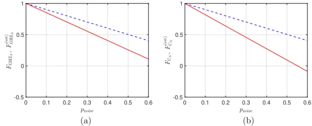
where 1 is the identity matrix, p_noise is the fraction of the noise, and we considered a system of N qudits with a dimension d. It is important that the witness used is able to detect not only the ideal state as entangled, but also the noisy state. The largest noise fraction pnoise for which the state is still detected as entangled is the robustness of the witness to noise. Alternatively, it is also called noise tolerance. Simple calculation shows that if the witness W detects|Ψias entangled (i.e., hWi_|Ψi<0) then a state of the type (2.1.7) is detected as entangled if

p_noise< hWi_|Ψi hWi_|Ψi− hWi_%

cm

. (2.1.9)

2.2 Using correlations to witness entanglement

Beside constructing entanglement witnesses, it is also important to find a way to measure them. For example, they can easily be measured by decomposing them into a sum of locally measurable terms [8]. Here we follow a different route. We will construct witness operators of the form

W_O :=O− inf

Ψ∈S

hΨ|O|Ψi

, (2.2.10)

whereSis the set of separable states, “inf” denotes infimum, andOis a fundamental quantum operator of a spin system which is easy to measure. In the general caseinfΨ∈ShΨ|O|Ψi is difficult, if not impossible, to compute [84, 85]. Thus we will concentrate on operators that contain only two-particle interactions and have certain symmetries. We derive a general method to find bounds for the expectation value of such operators for separable states. This method will be applied to spin lattices. We will also consider models with a different topology.

If observableOis taken to be the Hamiltonian then our method can be used for detect-

(22)

CHAPTER 2. ENTANGLEMENT DETECTION WITH CORRELATIONS 16 ing entanglement by energy measurement.² While our approach does not require that the system is in thermal equilibrium, it can readily be used to detect entanglement for a range of well-known systems in this case. The energy bound for separable states correspond to a temperature bound. Below this temperature the thermal state is necessarily entangled.

Let us consider first a simple example.

Example 2.2.1 For two-qubit separable states we have hσ⁽¹⁾_x σ_x⁽²⁾i+hσ_y⁽¹⁾σ_y⁽²⁾i+

σ⁽¹⁾_z σ_z⁽²⁾

≤1, (2.2.11)

while the maximum of the left-hand side of Eq. (2.2.11)for entangled quantum states is 3.

Proof. Let us consider first pure two-qubit product states of the form |ψ₁i ⊗ |ψ₂i.

Then, for such states we have

hσ_l⁽¹⁾σ⁽²⁾_l i=hσ_l⁽¹⁾ihσ⁽²⁾_l i (2.2.12) forl =x, y, z.Hence, the left-hand side of Eq. (2.2.11) can be written as a scalar product of two vectors

hσ_x⁽¹⁾σ⁽²⁾_x i+hσ⁽¹⁾_y σ_y⁽²⁾i+

σ_z⁽¹⁾σ⁽²⁾_z

=~v₁·~v₂, (2.2.13) where

~ v_n=





 hσx⁽ⁿ⁾i hσy⁽ⁿ⁾i hσz⁽ⁿ⁾i





 (2.2.14)

for n= 1,2. Finally, applying the Cauchy-Schwarz inequality we get

~

v₁~v₂ ≤ |~v₁||~v₂|= 1. (2.2.15) With that, we proved Eq. (2.2.11) for pure product states. Keeping in mind that separable states are the mixtures of product states, Eq. (2.2.11) is also valid for separable states

given in Eq. (2.1.2).

After the simple example, we consider spin lattice Hamiltonians. Calculations similar to this one are widely used in statistical physics, however, we still think that it will help to understand the basic goals of entanglement theory by connecting it to other areas of physics. We would like to find the minimal expectation value of such Hamiltonians for product states. The calculations can be simplified if the lattice can be divided into two sublattices, Aand B, such that every correlation term involves one spin component from

2Independently, a pre-print with a similar approach has appeared: Č. Brukner and V. Vedral, quant- ph/0406040.

(23)

0000 00 1111 11

000000 000 111111 111 000000

000 111111 111

0000 00 1111 11

00000000000000000 11111111111111111

0000 00 1111 11

0000 00 1111 11 0000 00 1111 11 000000 000 111111 111 000000 000 111111 111

00000000000000000 11111111111111111

00000000000000000 11111111111111111 00000000000000000 11111111111111111 00000000000000000 11111111111111111

0000 00 1111 11 000000

1111 11

0000 1111 0000 00 1111 11

000000 000 111111 111 000000 111111

000000 000 111111 111

0000 00 1111 11

000000 000 111111 111 000000

1111 11 000000

111111

00000000 0000 11111111 1111

000000 111111

000000 000 111111 111000000

1111 11 00000000 0000 11111111 1111

0000 1111

0000 00 1111 11

00000000 11111111 0000 00 1111 11 0000

00 1111 11

0000 1111

000000 000 111111 111

0000 00 1111 11

(a) (b)

(c) (d)

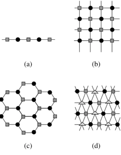
Figure 2.2: Some of the most often considered lattice models: (a) Chain, (b) two- dimensional cubic lattice, (c) hexagonal lattice and (b) triangular lattice. Different sym- bols at the vertices indicate a possible partitioning into sublattices. Figure is taken from Ref. [67].

sublatticeA and another one from sublatticeB.Such sublattices are shown in Fig. 2.2. If we also assume that all interaction terms are the same then we can write the expectation value of the Hamiltonian for such systems as

hHi=X

k

f(~s_a_k, ~s_b_k), (2.2.16) wheref is some two-spin function, and a_k andb_k denotes the indices of spins of sublattice A and B, respectively. The minimum over product states can be obtained as

Ψ1⊗Ψmin₂⊗...⊗Ψ_NhHi= min

{~sk}^N_k=1,|~sk|=1

X

k

f(~sa_k, ~sb_k). (2.2.17) It is possible to minimize the terms in Eq. (2.2.17) idependently, hence we arrive at

Ψ1⊗Ψmin2⊗...⊗ΨN

hHi=N_corr min

~

s^m,|~s^m|=1f(~s^A, ~s^B), (2.2.18) where N_corr is the number of correlation terms.

Finally, we need the minimum of hHi for separable states. Since separable states are just mixtures of product states, and the expectation value is hHi = Tr(%H) is linear in

%, the bound we obtain in Eq. (2.2.18) is also valid for separable states. Hence, if hHi is lower than this minimum, then the quantum state must be entangled. This way we can

(24)

0 5 0

5 0

0.1 0.2

k_BT/J B/J

E_F(B,T)

0

5 0

5 0 0.05 0.1

kBT/J x EF(B,T)

B/Jx

(a) (b)

Figure 2.3: (a) Heisenberg chain of 8spins. Nearest-neighbor entanglement as a function of magnetic field B and temperature T. (b) The same for an Ising spin chain. Here k_B is the Boltzmann constant, J and J_x are coupling constants. Light color indicates the region where entanglement is detected by our method. Figure is taken from Ref. [67].

detect entanglement based on energy measurement. With the formalism of Sec. 2.1.4, we can say that

W =H−N_corr min

~s^m,|~s^m|=1f(~s^A, ~s^B), (2.2.19) is an entanglement witness.

If the nondegenerate ground state or theT = 0thermal state of a system is entangled, then it is expected that the thermal state remains entangled even at finite temperatures up to a temperature bound. Let us define the temperatureTE such that the energy of the thermal state equals to the bound obtained in Eq. (2.2.18), that is,

Tr

He^T^H^E Tr

e

H TE

=N_corr min

~s^m,|~s^m|=1f(~s^A, ~s^B). (2.2.20) For T < T_E the thermal state will have lower energies than the bound (2.2.18), hence it must be entangled. It is straightforward to calculate T_E based on our approach. We add that we do not claim that the system is separable for all T > T_E.

2.3 Entanglement detection with well-known spin Hamil- tonians

Let us consider an anti-ferromagnetic Heisenberg Hamiltonian with periodic boundary conditions on a d-dimensional cubic lattice

H_H:=X

hk,li

σ_x^(k)σ_x^(l)+σ_y^(k)σ_y^(l)+σ_z^(k)σ_z^(l)+Bσ_z^(k). (2.3.21)

(25)

CHAPTER 2. ENTANGLEMENT DETECTION WITH CORRELATIONS 19 The strength of the exchange interaction is set to be J = 1, B is the magnetic field, and hk, lidenotes spin pairs connected by an interaction. The expectation value of Eq. (2.3.21) for separable states is bounded from below

hH_Hi ≥E_H,sep:=

−dN[(B/d)²/8 + 1] if |B/d| ≤4,

−dN(|B/d| −1) if |B/d|>4, (2.3.22) where N is the total number of spins. This bound was obtained using two sublattices, minimizing the expression f_H(~sÂ, ~s^B) :=~sÂ~s^B+B(sÂ_z +s^B_z)/(2d). Based on this E_H,sep = dNinf[f_H].³

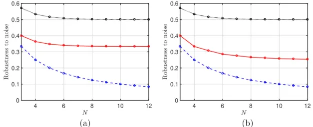
Another important question is how the temperature boundTE depends on the number of particles. For the Heisenberg model of even number of spins with B = 0 this temperature decreases slowly with N and saturates at T ≈ 3.18. Refs. [86, 87] find the same temperature bound for nonzero concurrence for an infinite system.

For the XY Hamiltonian on a d-dimensional cubic lattice with periodic boundary conditions

H_XY :=X

hk,li

J_xσ_x^(k)σ_x^(l)+J_yσ_y^(k)σ^(l)_y +B

N

X

k

σ^(k)_z (2.3.23) the energy of separable states is bounded from below as

hHXYi ≥EXY,sep :=

−dN M 1 +b²/4

if b≤2,

−dN M b if b >2. (2.3.24) HereJ_xandJ_Y are the nearest-neighbor coupling along thexandydirection, respectively.

B is the magnetic field, M := max(|J_x|,|J_y|) and b := |B|/M/d. This bound is simply the mean-field ground state energy. It was obtained using two sublattices and minimizing f_XY(~sÂ, ~s^B) := J_xsÂ_xs^B_x +J_ysÂ_ys^B_y +B(sÂ_z +s^B_z)/(2d).

A one-dimensional spin-1/2 Ising chain is a special case of an XY lattice withJ_x = 1 and J_y = 0. Fig. 2.3(b) shows the nearest-neighbor entanglement as a function of B and T for this system. According to numerics, T_E (computed for B = 1) decreases with increasing N. For N =∞we obtain T_E ≈0.41[88].

3If the number of sites along one dimension is odd, then a lattice with periodic boundary conditions cannot be partitioned into two sublattices such that neighboring sites correspond to different sublattices.

In this caseEsep given here is still a lower bound for the energy of separable states, but not necessarily the highest possible lower bound.

(26)

2.4 Connected work

We review some works connected to this topic. A similar approach has been reported in independent works in Ref. [89, 90]. Optimal temperature bounds have been calculated in Ref. [91]. References [78, 79] consider the detection of various forms of multipartite entanglement, described in Sec. 2.1.3, with a similar approach.

(27)

Chapter 3 Entanglement detection close to graph states

In this Chapter, we consider detection of multipartite entanglement close to graph states, which also include cluster states and GHZ states described in Refs. [39, 41, 69]. We present criteria that detect any type of entanglement, as well as criteria that detect only genuine multipartite entanglement. We also discuss how to estimate the fidelity with respect to such states based on Refs. [39, 41].

3.1 Background

3.1.1 GHZ states, as stabilizer states

There are various quantum states that appear often in experiments. One of them is the Greenberger-Horne-Zeilinger (GHZ) state [14] given in Eq. (1.1.3), which is the superposition of two states: all atoms in state ’0’ and all atoms in state ’1’. For large number of particles, this is the superposition of two macroscopically different states, i.e., a Schrödinger-cat state.

We introduce very briefly thestabilizer theory[92], which will be used for entanglement detection. This theory already plays a determining role in quantum information science.

Its key idea is describing the quantum state by its so-called stabilizing operators rather than the state vector. This works as follows: An observable S_k is a stabilizing operator of anN-qubit state |ψiif the state |ψi is an eigenstate of S_k with eigenvalue 1

Sk|ψi=|ψi. (3.1.1)

(28)

CHAPTER 3. ENTANGLEMENT DETECTION CLOSE TO GRAPH STATES 22 Many highly entangled N-qubit states can be uniquely defined byN stabilizing operators which are locally measurable, i.e., they are products of Pauli matrices.

We now show how the stabilizer theory can be used to give a set of correlations that determine the GHZ state uniquely. AnN-qubit GHZ state is given by Eq. (1.1.3). Besides this explicit definition one may define the GHZ state also in the following way: Let us look at the observables

S₁^(GHZ^N⁾ :=

N

Y

k=1

X^(k),

S_k^(GHZ^N⁾ := Z^(k−1)Z^(k) for k = 2,3, ..., N, (3.1.2) where X^(k), Y^(k), and Z^(k) denote the Pauli matrices acting on the k-th qubit. Now we can define the GHZ state as the state|GHZNi which fulfills

S_k^(GHZ^N⁾|GHZ_Ni=|GHZ_Ni (3.1.3) for k = 1,2, ..., N. One can straightforwardly calculate that the GHZ state is uniquely defined by Eq. (3.1.3). From a physical point of view the definition via Eq. (3.1.3) stresses that the GHZ state is uniquely determined by the fact that it exhibits perfect correlations for the observablesS_k^(GHZ^N⁾.

Note that|GHZ_Niis stabilized not only byS_k^(GHZ^N⁾, but also by their products. These operators, all having perfect correlations for a GHZ state, form a group called stabilizer [92]. This 2^N-element group of operators will be denoted by S^(GHZ^N⁾. The operators S_k^(GHZ^N⁾ are the generators of this group.

3.1.2 Cluster states and graph states

Cluster states are multipartite states arising naturally in Ising spin systems. In the two- dimensional case, they can be used for measurement based quantum computing as a resource [17].

For simplicity let us consider a one-dimensional cluster state defined in Eq. (1.1.6). One can use the stabilizer theory described in Sec. 3.1.1 to define cluster states. In this case, a cluster state |C_Ni is defined to be the state fulfilling the equations |C_Ni = S_k^(C^N⁾|C_Ni with the following stabilizing operators

S₁^(C^N⁾ := X⁽¹⁾Z⁽²⁾,

S_k^(C^N⁾ := Z^(k−1)X^(k)Z^(k+1);k = 2,3, ..., N −1,

S_N^(C^N⁾ := Z^(N−1)X^(N⁾. (3.1.4)

(29)

CHAPTER 3. ENTANGLEMENT DETECTION CLOSE TO GRAPH STATES 23 Analogously to the case of GHZ states described in Sec. 3.1.1, the cluster state is uniquely given by the N stabilizing operators (3.1.4).

Let us now describe graph states. They are the generalizations of cluster states [93].

A graph state corresponds to a graph G consisting of N vertices and some edges. The connectivity of this graph is defined by N(i), which gives the set of neighbors for vertex i. Let us define for each vertex a locally measurable observable

S_k^(G^N⁾ :=X^(k) Y

l∈N(k)

Z^(l). (3.1.5)

A graph state |GNi of N qubits is now defined to be the state which has the operators S_k^(G^N⁾ given in Eq. (3.1.5) as stabilizing operators. This means that the S_k^(G^N⁾ have the state |G_Ni as an eigenstate with eigenvalue +1,

S_k^(G^N⁾|G_Ni=|G_Ni. (3.1.6) We can see that cluster states correspond to graph states with

N(1) = {2},

N(n) = {n−1, n+ 1}, forn = 2,3, ..., N −1,

N(N) = {N −1}. (3.1.7)

3.1.3 Local decomoposition of entanglement witnesses

An entanglement witness W is typically a multipartite operator. In principle, it is an observable, and can be measured. In practice, it is very difficult to measure a multipartite operator. Fortunately, we do not need a von Neumann measurement ofW, we need only its expectation value. hWi can be obtained from a series of correlation measurements using the local decomposition

W =X

k

c_kA⁽¹⁾_k ⊗A⁽²⁾_k ⊗...A^(N_k ⁾, (3.1.8)

where N is the number of parties and A⁽ⁿ⁾_k are operators acting on party (n). Then,hWi is obtained as a weighted average of the expectation values of correlation measuements

hWi =X

k

ck

D

A⁽¹⁾_k ⊗A⁽²⁾_k ⊗...A^(N)_k E

. (3.1.9)

(30)

CHAPTER 3. ENTANGLEMENT DETECTION CLOSE TO GRAPH STATES 24

3.1.4 Local measurement settings

Based on the previous section, one might think that the experimental effort needed for measuring such an operator is characterized by the number of correlation terms we need for a decompositon. In fact, this is not the case. The experimental effort needed for measuring a witness can be characterized by the number of local measurement settings needed for its implementation [83, 94].

A local measurement setting

L={O^(k)}^N_k=1 (3.1.10)

consists of performing simultaneously the von Neumann measurements O^(k) on the corresponding parties. By repeating the measurements many times one can determine the probabilities of the possible outcomes. Given these probabilities it is possible to compute all two-point correlations hO^(k)O^(l)i, three-point correlations hO^(k)O^(l)O^(m)i, etc. Hence, there are several correlation terms that can be measured with a single setting.

Optimal decompositions for various system sizes and operators has been intensively studied [95–97]. The number of measurement settings needed to decompose any projector to an N-qubit symmetric state is at most (N²+ 3N + 2)/2[71].

3.2 Detection of entanglement

Based on Sec. 3.1.1, we construct our witness from two locally non-commuting stabilizing operators:

Observation 3.2.1 A witness detecting entanglement around an N-qubit GHZ state is W_m^(GHZ^N⁾ :=1−S₁^(GHZ^N⁾−S_m^(GHZ^N⁾, (3.2.11) where m= 2,3, ..., N.

Proof. The proof is based on the Cauchy-Schwarz inequality. Using this andhX⁽ⁱ⁾i²+ hZ⁽ⁱ⁾i² ≤1, for pure product states we obtain

hS₁^(GHZ^N⁾i+hS_m^(GHZ^N⁾i=

=hX⁽¹⁾ihX⁽²⁾i...hX^(N⁾i+hZ^(m−1)ihZ^(m)i

≤ |hX^(m−1)i| · |hX^(m)i|+|hZ^(m−1)i| · |hZ^(m)i|

≤ q

hX^(m−1)i²+hZ^(m−1)i² q

hX^(m)i²+hZ^(m)i²

≤1. (3.2.12)

(31)

CHAPTER 3. ENTANGLEMENT DETECTION CLOSE TO GRAPH STATES 25 It is easy to see that the bound is also valid for mixed separable states.

This proof can straightforwardly be generalized to arbitrary two locally non-commuting elements of the stabilizer. Using the definitions of Sec. 3.1.2, a derivation similar to the one above yield the following.

Observation 3.2.2 A witness detecting entanglement around anN-qubit cluster state is W_m^(C^N⁾ :=1−S_m^(C^N⁾−S_m+1^(C^N⁾, (3.2.13) where m= 1,3, ..., N −1.

Proof. The proof is analogous to the poof of the previous Observation 3.2.1.

3.3 Detection of multipartite entanglement

The measurement of the fidelity with respect to some pure quantum state, and the detection of genuine multipartite entanglement are needed in numerous quantum experiments (e.g., Refs. [40, 44, 98]). In most of these experiments, only local measurements can be carried out. For such systems, many methods need a measurement effort increasing exponentially with the number of qubits [39]. This also means that measuring the quantum fidelity and measuring witness operators is impractical in many cases apart from very small particle numbers. Hence, it has been noted that it is not clear that entanglement witnesses have really an advantage over full state tomography (e.g., Ref. [83]). It seems that we cannot obtain any useful information in an experiment about the quantum state prepared. Indeed, there is no a priori reason that the detection of multipartite entanglement is possible in a scalable way with local measurements.

In this section, we will present efficient methods, which need few local measurements, to detect genuine multipartite entanglement in the vicinity of stabilizer states, and also for obtaining a very good lower bound on the fidelity. Next, we present efficient witnesses for GHZ states.

Observation 3.3.1 The following entanglement witness detects genuine N-qubit entanglement for states close to an N-qubit GHZ state:

W_GHZ_N := 31−2

S₁^(GHZ^N⁾+1

2 +

N

Y

k=2

S_k^(GHZ^N⁾+1 2

. (3.3.14)