Kibble–Zurek mechanism in the Ising Field Theory K. Hódsági

(1)

Kibble–Zurek mechanism in the Ising Field Theory

K. Hódsági^1* and M. Kormos²

1BME-MTA Statistical Field Theory Research Group, Institute of Physics, Budapest University of Technology and Economics,

1111 Budapest, Budafoki út 8, Hungary

2 MTA-BME Quantum Dynamics and Correlations Research Group, Budapest University of Technology and Economics,

1111 Budapest, Budafoki út 8, Hungary

*hodsagik@phy.bme.hu September 11, 2020

Abstract

The Kibble–Zurek mechanism captures universality when a system is driven through a continuous phase transition. Here we study the dynamical aspect of quantum phase transitions in the Ising Field Theory where the quantum critical point can be crossed in different directions in the two-dimensional coupling space leading to different scaling laws. Using the Truncated Conformal Space Approach, we investigate the microscopic details of the Kibble–Zurek mechanism in terms of instantaneous eigenstates in a genuinely interacting field theory. For different protocols, we demonstrate dynamical scaling in the non- adiabatic time window and provide analytic and numerical evidence for specific scaling properties of various quantities. In particular, we argue that the higher cumulants of the excess heat exhibit universal scaling in generic interacting models for a slow enough ramp.

1 Introduction

The Kibble–Zurek mechanism (KZM) describes the dynamical aspects of phase transitions and captures the universal features of nonequilibrium dynamics when a system is driven slowly across a continuous phase transition. The original idea is due to Kibble, who studied cosmological phase transitions in the early Universe [1, 2]. He showed that as the Universe cools below the symmetry breaking temperature, instead of perfect ordering, domains form and topological excitations are created. Not much later Zurek pointed out that this phenomenon can be observed in condensed matter systems as well, and that the density of defects depends on the cooling rate [3, 4]. The physical mechanism originates in the fact that at a critical point both the correlation length and the correlation time (relaxation time) diverge, leading to an inevitable breakdown of adiabaticity. As a consequence, the final state will not be perfectly ordered but will consist of domains with different symmetry breaking orders separated by defects or domain walls. However, in the process a typical time scale and a corresponding length scale emerges related to the instant when the system deviates from the adiabatic course. These quantities, diverging as the rate at which the phase transition is crossed approaches zero, are the only scales in the problem.

As a consequence, the density of domain walls as well as other quantities obey scaling laws in terms of the speed of the ramp.

It is a natural question whether the same phenomena occur also at zero temperature, i.e.

for quantum critical points. A systematic study of the KZM in quantum phase transitions started with the works [5–8]. Quantum phase transitions are different from transitions at finite temperature: they correspond to a qualitative change in the ground state of a quantum system and are driven by quantum fluctuations. Importantly, the time evolution

(3)

is unitary and there is no dissipation. In spite of these differences, the scaling behaviour essentially coincides with the classical case [5–10]. The scaling behaviour was extended to other observables beyond the defect density to correlation functions [11–13], entanglement entropy [13–15], excess heat [16–18], and also to different ramp protocols [10, 16, 19–21], including quenches from the ordered to the disordered phase. The scaling laws can also be derived using the framework of adiabatic perturbation theory [7, 16, 17, 19, 22–25]. The reader interested in the KZM in the context of quantum phase transitions is referred to the excellent reviews [26–28].

The simplest approximation which leads to the right scaling exponents assumes that when adiabaticity is lost, the system becomes completely frozen and reenters the dynamics only some time after crossing the critical point. This freeze-out scenario or impulse approximation has been refined recently by taking into account the actual evolution of the system in the non-adiabatic time window [15, 29–35]. Since the Kibble–Zurek length and time scales are the only relevant scales, the non-adiabatic evolution features dynamical scaling, i.e. the time dependence of various observables is given by scaling functions. This can also be understood from an adiabatic renormalization group approach [20, 21].

The Kibble–Zurek mechanism was also extended beyond the mean values to the full statistics of observables. The number distribution of defects was computed in the Ising chain [13, 36] and was argued to exhibit universality [37]. Similarly, the work statistics and its cumulants were also studied and found to satisfy scaling relations [38–40].

The quantum KZM has been investigated experimentally in cold atomic systems [41–

45], including the dynamical scaling [46, 47] and very recently, the number distribution of the defects [48].

The various facets of the quantum KZM was demonstrated and analysed on the quantum Ising chain [6–8, 10, 13, 30, 33, 35, 36, 39, 40, 49–52], the XY spin chain [11, 12, 53] or other exactly solvable systems [15, 31, 50, 54, 54–56] (see however e.g. [9, 18, 34, 57, 58]).

Most studies focused on spin chains or other lattice systems, while field theories received less attention. Notable exceptions are Refs. [31, 54–56] and applications of the adiabatic perturbation theory approach to the sine–Gordon model [17, 23, 59]. The KZM in the field theory context also appeared in the context of holography [60–64].

In this work we aim to study different aspects the quantum Kibble–Zurek mechanism in a simple but nontrivial field theory, the paradigmatic Ising Field Theory. This theory is an ideal testing ground as it allows one to study both free and genuinely interacting integrable systems. Our motivation for this choice is twofold. First, we wish to study the KZM in a field theory at the microscopic level of states. Second, we would like to test the recent predictions for the universal dynamical scaling and the scaling behaviour of the higher cumulants of the work in an interacting model.

As we focus on an interacting theory, we need to use a numerical tool for our studies. We use a nonperturbative numerical method, the Truncated Space Approach [65–67]. Apart from its long-standing history to capture equilibrium properties of perturbed conformal field theories [68–80], recent applications demonstrate that it is capable to describe non- equilibrium dynamics in different models [81–86]. This approach gives us access to the microscopic data and full statistics of observables so we can investigate the KZM at work at the lowest level, and being nonperturbative and independent of integrability, it allows us to study the dynamics of the interacting field theory.

The paper is organised as follows. In Sec. 2 we outline the context of our work and review the scaling laws predicted by the Kibble–Zurek mechanism for quantum phase transitions. We proceed by defining the model in which we study the Kibble–Zurek mechanism and discuss the adiabatic perturbation theory that provides another viewpoint on the scaling laws. The main body of the text presents an in-depth analysis of the Kibble–Zurek

(4)

mechanism in the Ising Field Theory. In Sec. 3 we explore the implications of driving a system across a critical point on the statistics of work function and examine the behaviour of energy eigenstates to check the hypothesis of the KZM at a fundamental level. Sec.

4 discusses the dynamical critical scaling with the time and length scales corresponding to the deviation from the adiabatic course and demonstrates that the KZ scaling can be observed in the interacting E₈ model. In Sec. 5 we show that the appearance of the scaling connected to the Kibble–Zurek mechanism is not limited to local observables but it is present also in higher cumulants of the distribution of the excess heat. Finally, Sec. 6 finishes the paper with concluding remarks and possible future directions. Technical details concerning the relation of the adiabatic perturbation theory to theE₈ model, the scaling limit of the analytic solution of the dynamics on the transverse field Ising chain and the applicability of TCSA to the study of KZM are discussed in the Appendices.

2 Model and methods

In this section we describe the context of our work by introducing the concepts of the universal non-adiabatic behaviour that manifests itself in power-law dependence of several quantities on the time scale of the non-equilibrium ramp protocol, known under the name of Kibble–Zurek scaling. Then we discuss the model in which we study the KZ scaling, the Ising Field Theory which is the low energy effective theory of the transverse field Ising chain in the vicinity of its critical point. After introducing its main properties, we address the methods that are going to be used to examine the Kibble–Zurek scaling. In the limit of slow ramps, one can employ a perturbative approach, the adiabatic perturbation theory (APT) to investigate the time evolution. We give an overview of this approach, focusing on its application to universal dynamics near quantum critical points. The non-equilibrium dynamics of the Ising Field Theory is amenable to an efficient numerical non-perturbative treatment based on the truncated conformal space approach (TCSA), which we review briefly at the end of the section.

2.1 The Kibble–Zurek mechanism

In this section we summarise the KZ scaling laws in a fairly general fashion. Let us consider a perturbation of a quantum critical point (QCP) by some operator with scaling dimension∆.The strength of the perturbation is characterised by a coupling constant δ withδ = 0 corresponding to the critical point. Imagine that we prepare the system in its ground state and drive it through its QCP by changing δ in time, i.e. by performing a ramp. For the sake of generality, we consider ramps that cross the phase transition in a power-like fashion, i.e. near the QCP

δ=δ0

t τ_Q

a

sgn(t), (2.1)

whereτ_Qis the rate of the quench. The essence of the KZM is that due to the divergence of the relaxation time of the system at the QCP, known as critical slowing down, the system cannot follow adiabatically the change no matter how slow it is, and falls out of equilibrium meaning that it will be in an excited state with respect to the instantaneous Hamiltonian.

However, due to universality near the critical point the time and length scales corresponding to the deviation from the adiabatic course depend on the quench rateτ_Q as a power-law.

The scaling can be determined by the following simple argument. The correlation length diverges in the phase transition corresponding to this particular perturbation asξ ∝δ^−ν

(5)

whereν is the standard equilibrium critical exponent related to the scaling dimension ∆ of the perturbing operator byν = (2−∆)⁻¹.Similarly, the correlation or relaxation time diverges as ξ_t ∝ξ^z ∝ δ^−νz, where z is the dynamical critical exponent. If the change of ξ_twithin a relaxation time is much smaller than the relaxation time itself, ξ˙_tξ_tξ_t,then the evolution is adiabatic. This is the case for times

|t| τKZ≡(aνz)^aνz+1¹ τ_Q δ₀^1/a

! ^aνz

aνz+1

. (2.2)

However, once we reacht≈ −τ_KZ,the rate of change of the correlation time becomesξ˙t≈1 and the evolution becomes non-adiabatic. At this Kibble–Zurek timeτ_KZ,the correlation time scales with the quench rateτ_Q asτ_KZ itself:

ξ_t(−τ_KZ)∝ τ_Q δ₀^1/a

!_aνz+1^aνz

∝τ_KZ. (2.3)

The first formulation of Kibble–Zurek arguments depicted the non-adiabatic interval of time evolution as a simple freeze-out referring to the assumption that the state is literally frozen in the non-adiabatic regime t ∈ [−τ_KZ, τ_KZ]. At t = τ_KZ on the other side of the QCP, the system finds itself in an excited state with correlation lengthξ_KZ=ξ(−τ_KZ). If the system is now in the ordered phase, it implies that the typical linear size of the ordered domains are ∼ξ_KZ, so the density of excitations corresponding to defects (domain walls) in spatial dimensiondis

nex ∝ξ^−d_KZ∝ τQ

δ^1/a₀

!− ^aνd

aνz+1

. (2.4)

Recently, the freeze-out scenario was refined by taking into account the evolution of the system and change of the correlation length in the time interval−τ_KZ< t < τ_KZ[29–31,33].

The latter is caused by moving domain walls at the typical velocity corresponding to their typical wave number k ∼ ξ_KZ⁻¹ and energy ε(k) ∼ k^z ∼ ξ_KZ^−z. The velocity of this “sonic horizon” [33] isv=ε⁰(k)∼k^z/k∼ξ_KZ^1−z.The correlation length att=τ_KZ is then

ξ(τ_KZ) =ξ(−τ_KZ) + 2v2τ_KZ=ξ_KZ(1 + 4τ_KZ/ξ_KZ^z ) =ξ_KZ(1 + 4τ_KZ/ξt(−τ_KZ)) (2.5) which, due to Eq. (2.3), is proportional toξ_KZ.This means thatξ_KZis still the only relevant length scale so the scaling laws are not altered.

Still, nontrivial predictions can be made concerning the non-adiabatic or impulse region

−τ_KZ < t < τ_KZ [31, 33, 34] due to the fact that the KZ time and correlation length, τ_KZ andξ_KZ,are the only relevant scales for a slow enough ramp protocol. Consequently, time- dependent correlation functions are described in terms of scaling functions of the rescaled variablest/τ_KZ and x/ξ_KZ in the KZ scaling limit τ_KZ→ ∞.For example, one- and two- point functions of an operatorO_∆_O with scaling dimension∆_Otake the form in the impulse regimet∈[−τ_KZ, τKZ]

hO_∆_O(x, t)i=ξ_KZ^−∆^OFO(t/τKZ),

O_∆_O(x, t)O_∆_O(0, t⁰)

=ξ_KZ^−2∆^OGO

t−t⁰ τ_KZ , x

ξ_KZ

, (2.6) whereF and Gare scaling functions depending on the operatorO and we assumed trans- lational invariance. Note that for one-point functions the scaling holds in the adiabatic regime t <−τ_KZ as well, since there the expectation value depends only on the distance from the critical point, which is the function of the dimensionless timet/τ_Q:

hO_∆_O(x, t)i ∝ξ(t)^−∆^O ∝ t

τ_Q aν∆O

∝ t

τ_KZ aν∆O

τ_KZ^−∆^O^/z, (2.7)

(6)

where in the last step we used the relation (2.2).

Considering the generic nature of arguments presented above it is tempting to ask how precisely they describe the actual non-equilibrium dynamics of quantum systems.

The scaling relations are supported by exact calculations in the free fermionic Ising chain where the dynamics of low-energy modes can be mapped to the famous Landau–Zener transition problem [5, 8, 33, 87]. In other quantum phase transitions, when exact solutions are not available, the scaling can be analysed by a perturbative expansion in the derivative of the time-dependent coupling as a small parameter. This approach that uses adiabatic perturbation theory predicts the same scaling as the arguments of Kibble–Zurek mechanism in several models besides the Ising chain [7, 17, 19, 23]. This formalism is useful to apply the generic scaling arguments outside the non-adiabatic regime for quantities that are beyond the scope of the initial formulation of KZM [40]. Together with the non-perturbative numerical method employed in our work it can be used to establish the validity of the scaling relations listed above for an interacting model as well.

To do so, we have to address the question of finite size effects. These are of importance due to the fact that the TCSA method requires finite volume, while the arguments presented above make use of a divergent length scale ξKZ. Clearly, finite volume can bring about adiabatic behaviour if

ξKZ'L ⇒ (τQ/ξt)^aνz+1^aν 'L/ξ , (2.8)

whereξ and ξ_t are the correlation length and time at the initial state. If the quench rate τ_Q is significantly larger than this, the transition is adiabatic due to the fact that finite volume opens the gap. One way to compensate this effect is the rescaling of the volume parameter with the appropriate power of the quench rate [30]. However, if

τ_Q/ξ_t(L/ξ)^aνz+1^aν (2.9)

then the finite size effects are negligible. As we are going to illustrate in Sec. 3.3, we can set the parameters of the numerical TCSA method such that this relation is satisfied and there is no need to rescale the volume parameter.

2.2 KZM in the Ising Field Theory

After setting up the context of our work, we now turn to the model in consideration:

the Ising Field Theory that is the scaling limit of the critical transverse field Ising chain.

The Hamiltonian of the latter reads H_TFIC =−J X

i

σ_i^xσ^x_i+1+h_xX

i

σ^x_i +h_zX

i

σ_i^z

!

, (2.10)

whereσ_i^αwithα=x, y, zare the Pauli matrices at sitei,the strength of the ferromagnetic coupling J sets the energy scale, and hxJ and hzJ are the longitudinal and transverse magnetic fields, respectively. We set periodic boundary conditions,σ_L+1^α =σ₁^α.The model is fully solvable in the absence of the longitudinal field, h_x = 0, when it can be mapped to free Majorana fermions via the nonlocal Jordan–Wigner transformation. The Hilbert space is composed of two sectors based on the conserved parity of the fermion number. The fermionic Hamiltonian will be local provided we impose anti-periodic boundary conditions for the fermionic operators in the even Neveu–Schwarz (NS) sector and periodic boundary conditions in the odd Ramond (R) sector.

The transverse field Ising model is a paradigm of quantum phase transitions: in infinite volume, forhz<1the ground state manifold is doubly degenerate, spontaneous symmetry

(7)

Figure 2.1: Phase diagram of the Ising Field Theory. The couplingsM and h characterise the strengths of the perturbations of thec= 1/2conformal field theory by its two relevant operators,εandσ.The KZM is studied for ramps along the integrable directions indicated by the coloured arrows.

breaking selects the states(|0i_NS± |0i_R)/√

2 with finite magnetisationhσi=±(1−h²_z)^1/8 (here|0i_NS/Rare the ground states in the two sectors). In finite volume, there is an energy split between the states|0i_NSand|0i_R which is exponentially small in the volume, and the ground state is |0i_NS. In the paramagnetic phase for h_z > 1, the ground state is always

|0i_NS and the magnetisation vanishes. The quantum critical point (QCP) separating the ordered and disordered phases is located at hz = 1, which can also be seen from the behaviour of the gap, ∆ = 2J|1−h_z|, vanishing at the QCP. In the ferromagnetic phase, the massive fermionic excitations can be thought of domain walls separating domains of opposite magnetisations, and with periodic boundary conditions their number is always even¹. In the paramagnetic phase the excitations are essentially spin flips in thezdirection.

Forh_x 6= 0the model is not integrable² for any value ofh_z,but features weak confinement: the nonzero longitudinal field splits the degeneracy between the two ground states with an energy difference proportional to the system size. The domain walls cease to be freely propagating excitations, as the energy cost increases with the distance between two neighbouring domain walls that have a domain of the wrong magnetisation between them.

The new excitations are a tower of bound states, sometimes called ‘mesons’ in analogy with quark confinement in the strong interaction.

The low energy effective theory describing the model near the critical point is the Ising field theory, obtained in the scaling limit J → ∞, a → 0, h_z → 1 such that speed of light c_` = 2J a and the gap ∆ = 2J|1−h_z| are fixed (a is the lattice spacing). The critical point corresponds to the theory of a free massless Majorana fermion, which is also one of the simplest conformal field theories (CFT). Due to relativistic invariance, the dynamical critical exponent isz = 1. The two relevant operators at the quantum critical point are the magnetisationσ (scaling dimension1/8) and the so-called ‘energy density’ε (scaling dimension1), corresponding to the longitudinal and transverse magnetic fields in

1This is true even in the Ramond sector, as|0iRcontains a zero-momentum particle.

2Theσ_i^xoperators are nonlocal in terms of the fermions so the Jordan–Wigner transformation does not lead to a local fermionic Hamiltonian.

(8)

the scaling limit. The Hamiltonian of the resulting field theory in finite volumeL is given by

H_IFT=H_FF+M 2π

Z L 0

ε(x)dx+h Z L

0

σ(x)dx . (2.11)

HereHFF is the Hamiltonian of the free massless Majorana fermion, a minimal CFT with central chargec = 1/2.The precise relations between the lattice and continuum versions of the longitudinal magnetic field and the magnetization operator are

σ(x=ja) = ¯sJ^1/8σ^x_j , (2.12)

h= 2¯s⁻¹J^15/8h_x, (2.13)

with¯s= 2^1/12e^−1/8A^3/2 whereA= 1.2824271291. . . is Glaisher’s constant.

For h = 0 the Hamiltonian describes the dynamics of a free Majorana fermionic field with mass |M| (we set the speed of light to one, c` = 1). We will refer to this choice of parameters in the M−h parameter plane of the theory (2.11) as the “free fermion line”

(see Fig. 2.1). The QCP at M = 0 separates the paramagnetic phase M > 0 from the ferromagnetic phase M < 0.The coupling is proportional to the mass gap and since the correlation length is the inverse of the gap,ν= 1.

Interestingly, there is another set of parameters that corresponds to an integrable field theory: M = 0 with h finite³. The spectrum of this theory can be described in terms of eight stable particles, the mass ratios and scattering matrices of which can be written in terms of the representations of the exceptional E₈ Lie group. From now on, we are going to refer to this specific set of parameters as the “E₈ integrable line” (see Fig. 2.1). The lightest particle with massm1 sets the energy scale which is connected to the couplingh as

m₁ = (4.40490857. . .)|h|^8/15. (2.14) The exponent reflects that along theE8 line (σperturbation)ν = 8/15andz= 1.Moving particle states are built up as combinations of particles with finite momenta from the same or different species. The masses of the these particle species can be expressed in terms of m₁ as [88]

m₂ = 2m₁cosπ

5 , m₃ = 2m₁cos π

30 , m₄ = 2m₂cos7π

30 , m₅= 2m₂cos2π 15 , m6= 2m2cos π

30 , m7 = 4m2cosπ 5cos7π

30 , m8 = 4m2cosπ 5cos2π

15 . (2.15) The exact relation betweenm₁ and the coupling constant h was derived in Ref. [89]. Due to the integrability of the model, the scatteringS-matrix involving all different species is also known exactly [88]. This, in particular, allows for the identification of multiparticle eigenstates in finite volume based on the volume dependence of their energy.

In the following we are going to consider ramp protocols along the integrable lines, indicated by the coloured arrows in Fig. 2.1. Using the terminology of Ref. [31], we distinguish protocols withλiandλ_fcorresponding to different phases of the model (ramp crossing the critical point), and protocols withλ_f = 0 (ramp ending at the critical point). We are going to refer to these two choices as trans-critical protocol (TCP) and end-critical protocol (ECP), respectively. Certain observables exhibit markedly different behaviour depending on the protocol [40], hence both of them are of interest.

3The lattice model is not integrable forhz = 1andhx 6= 0,this is a feature of the field theory in the scaling limit.

(9)

We focus our attention on linear ramps, where one of the couplings is varied such that the system reaches or crosses the critical point at a constant rate,

λ(t) =−λ₀ t

τ_Q, (2.16)

where λ stands for M or h and the other coupling is set to zero. τ_Q is the duration of the ramp that takes place in the time interval t ∈ [−τ_Q/2, τ_Q/2] for a TCP ramp and t∈[−τ_Q,0]for an ECP ramp.

Ramps along the free fermion line (h = 0) have been studied extensively, especially in the spin chain. The time evolution of the free fermion modes with different momentum magnitudes decouple and only modes of opposite momenta{k,−k}are coupled by the evolution equation. One can make progress either by invoking the Landau–Zener description of transitions between energy levels or by numerically solving the set of two differential equations. Even analytical solutions are known for various ramp profiles [26, 54]. These solutions can be simply generalised to the continuum field theory, providing us with an analytical tool to examine the KZ scaling and offering a benchmark for our numerical method. We refer the reader to Appendix B for the details.

The Kibble–Zurek mechanism is much less studied along the other integrable axis M = 0.As we noted above, in this direction ν= 8/15,so the KZ scaling is modified with respect to the well-investigated free fermion case. Although the model is integrable, the time evolution cannot be solved analytically, which highlights the importance of the non- perturbative numerical method that exploits the conformal symmetry of the critical model:

the Truncated Conformal Space Approach (TCSA). Nevertheless, standard KZ arguments rely only on typical energy and distance scales of the model, consequently they should apply regardless of the presence of interactions. The scaling arguments can be supported by the analysis of the exactly known form factors of the model in the context of the adiabatic perturbation theory, to which we turn now.

2.3 Adiabatic Perturbation Theory

The adiabatic perturbation theory (APT) is a standard approach to study the response to a slow perturbation [27, 90]. It was first used to describe the universal dynamics of extended quantum systems in the vicinity of a quantum critical point in Ref. [7]. Ever since the framework has become more elaborate by exploring the parallelism between APT and the Kibble–Zurek mechanism and generalising the arguments to a wider variety of scaling quantities in different models [16, 17, 19, 23–25, 40]. In particular, it has already been applied with success in an integrable field theory, the sine–Gordon model [17]. In our current work we carry out an analogous reasoning to explore the implications of the APT statements in theE8 Ising Field Theory. To this end, let us briefly sketch the basic concepts and assumptions underlying the framework of adiabatic perturbation theory as well as introduce some notations. Our discussion is based on the presentation of Ref. [24].

Assume that we want to solve the time-dependent Schrödinger equation:

ıd

dt|Ψ(t)i=H(t)|Ψ(t)i (2.17) in a time interval t ∈ [t_i, t_f]. Using the basis of eigenstates of H(t) that are going to be called instantaneous eigenstates|n(t)i,

H(t)|n(t)i=E_n(t)|n(t)i , (2.18) we can expand the time evolved state with coefficientsα_n(t):

|Ψ(t)i=X

n

α_n(t) exp{−ıΘ_n(t)} |n(t)i , (2.19)

(10)

where the dynamical phase factorΘ_n(t) =Rt

tiE_n(t⁰) dt⁰ is already included. The initial condition is that atti the system is in its ground state |0(t_i)i. Substituting this Ansatz into Eq. (2.17) yields a system of coupled differential equations for the coefficientsα_n(t). The resulting system of equations can be solved approximately forα_n(t) using a few assumptions. First, the explicit time-dependence of the Hamiltonian is due to a time-dependent coupling constant λ that couples to some perturbing operator V so H(t) = H₀ +λ(t)V. Second, λ(t) is a monotonous function of time, hence one can perform a change of variables, and it changes slowly (that is the adiabatic assumption) such thatλ˙ →0. Then the resulting expression can be expanded in terms of powers ofλ. Assuming there is no Berry˙ phase, the result up to leading order inλ˙ is

α_n(λ)≈ Z λ

λi

dλ⁰ n(λ⁰)

∂_λ⁰ 0(λ⁰)

exp

ı(Θ_n(λ⁰)−Θ₀(λ⁰)) , (2.20) where the dynamical phase with respect to the coupling isΘn(λ) =R_λ

En(λ⁰)/λ˙⁰dλ⁰ with λ=λ(t).Note that the phase factor exhibits rapid oscillations in the limitλ˙ →0. This can be exploited to identify the two possibly dominant contributions of integral Eq. (2.20) in this limit. First, a non-analytic part that comes from the saddle point of the phase factor at a complex value of couplingλ. It is exponentially suppressed with the inverse of the rate λ. Second, there are contributions coming from the boundaries of the integration domain˙ which can be obtained by integrating by parts and keeping terms to first order inλ˙ yields the result

α_n(λ_f)≈ıλ˙⁰hn(λ⁰)|∂_λ⁰|0(λ⁰)i E_n(λ⁰)−E₀(λ⁰) exp

ı(Θ_n(λ⁰)−Θ₀(λ⁰))

λf

λi

. (2.21)

This contribution can be viewed as a switch on/off effect as it is the consequence of a non- smooth start or end of the ramp: it is nonzero if the first time derivative of the coupling has a discontinuity at the initial or final times. Ifλ˙_i,f= 0 then one has to go to higher orders.

In general, a discontinuity in theath derivative brings about the scalingα∝τ_Q^−awith the time parameter of the ramp τQ [26]. We consider linear ramps (cf. Eq. (2.16)) so higher derivatives disappear and the small parameter of the perturbative expansion is1/τ_Q. We remark that Eq. (2.21) can be modified if the energy difference in the denominator vanishes at some time instant along the process, in that case the dependence ofα on λ˙ is subject to change (cf. Eq. (2.26) for low-momentum modes if the gap is closed).

The applicability of adiabatic perturbation theory, strictly speaking, requires that the overlap between the time-evolved state and the instantaneous ground state remains close to 1 [90]. This, however, imposes a constraint on the probability to be in an excited state rather than on the density of excitations. On the other hand, for quantum many-body systems in the thermodynamic limit the physical criterion for a perturbative treatment is to be in a low-density state [19]. Given that the Kibble–Zurek mechanism predicts that densities decay as a power law of the time parameterτ_Q, in the limit τ_Q → ∞the above approximations are justified and we can use Eq. (2.20) to examine the Kibble–Zurek scaling.

This reasoning predicts the correct scaling exponents in the transverse field Ising chain for various quantities [24, 40]. Let us illustrate how they work in the case of the density of defects n_ex after a linear ramp λ(t) = λ_i+ (λ_f−λ_i)t/τ_Q. The states of the Ising chain participating in the dynamics are products of zero-momentum particle pair states with momentumk, hence the defect density can be expressed as⁴

n_ex= lim

L→∞

2 L

X

k>0

|α_k|²= Z π

−π

dk

2π|α_k|², (2.22)

4We remark that in principle the normalization of the state should be taken into account, but it is1 up to first order in the perturbation theory.

(11)

whereα_k=α_k(λ_f) is the coefficient of a particle pair state|k,−kigiven by Eq. (2.20). To investigate the dependence onτ_Q it is practical to introduce the rescaled variables

η=kτ

ν 1+zν

Q , ζ =λτ

1 1+zν

Q . (2.23)

to remove the 1/τQ dependence from the exponent of Eq. (2.20). The heart of the APT treatment of KZ scaling lies at the observation that the matrix element and energy difference appearing in the expression ofα_ntake the following scaling forms:

E_k(λ)−E₀(λ) =|λ|^zνF(k/|λ|^ν) (2.24) h{k,−k}(λ)|∂λ|0(λ)i=λ⁻¹G(k/|λ|^ν), (2.25) with the asymptotic behaviourF(x)∝x^z and G(x) ∝x^−1/ν asx→ ∞. These considerations yield that

n_ex=τ⁻

ν 1+zν

Q

Z dη

2πK(η), (2.26)

with

K(η) =

Z ζ_f ζi

dζG(η/ζ^ν) ζ exp

ı

Z ζ ζi

dζ⁰ζ^0zνF(η/ζ^0ν)

2

. (2.27)

Eq. (2.26) is analysed in the limit τ_Q → ∞. In that case the limits of the integral over η are sent to ±∞ and one has to check whether the resulting integral converges or not.

Substituting Eqs. (2.24) and (2.25) one can perform the integral in (2.27) in the limit ηζ_i,f^ν to determine the asymptotic behaviour

K(η)∝η^β ≡η^−2z−2/ν. (2.28)

The criterion for convergence then is 2z+ 2/ν >1, or, equivalently _1+zν^ν <2 [24]. In the opposite case the integral is divergent, indicating that to discard the contribution from high-energy modes in the limit τQ→ ∞is not justified. The scaling brought about by all energy scales is quadraticτ_Q⁻² due to the discontinuity of λ, cf. Eq. (2.21). Consequently,˙ the case of equality _1+zν^ν = 2 distinguishes between the Kibble–Zurek scaling determined by the exponent ofτQ in Eq. (2.26) and the quadratic scaling.

2.3.1 Application to the Ising Field Theory

These are the key themes of adiabatic perturbation theory as applied to model the Kibble–Zurek mechanism. Now we are going to show that these considerations can be generalised to the two integrable directions of the Ising Field Theory. In the case of the free field theory the generalisation of the arguments above is straightforward and it yields the same result as for the free fermion Ising chain. To apply the reasoning to the E₈ integrable model requires a bit of extra work. The complications are mainly technical, details are presented in Appendix A. Here we would like to highlight the key assumptions of the arguments only.

There are several major differences between the free fermion and theE₈field theory: the spectrum of the latter exhibits eight stable stationary particles, moving particle states are built up by combining particles of various species. As a result, there are multiple kinds of many-particle states in contrast to the pair of a single particle species in the free field theory.

Interactions between particles modify the simplepn= 2πn/Lquantisation rule of momenta in finite volumeL, leading to a nontrivial density of states in momentum space. Eigenstates of the theory are asymptotic scattering states labelled by the relativistic rapidity variable

(12)

ϑ that is related to the energy and momentum of particle j as E_j = m_jcoshϑ_j and pj =mjsinhϑj.

To investigate the Kibble–Zurek scaling in this model we make several simplifying assumptions. First, we consider low-density states which is justified in the limit τ_Q → ∞.

Apart from being a necessary assumption to use the framework of adiabatic perturbation theory, it sets the ground for our second assumption: that is, we assume that the contribution from one- and two-particle states contribute dominantly to intensive quantities such as the defect and energy density. In contrast to the free fermion case, the time-evolved state in theE₈ model includes contributions from multiparticle states that do not factorise exactly to a product of particle pairs. On the other hand, the many-particle overlap functions still satisfy the pair factorisation up to a very good approximation given that the energy density of the non-equilibrium state is low [82, 91] compared to the natural scale set by the final mass gap. Intuitively, the essence of this approximation is that due to large interparticle distance, the interactions between particles located far from each other can be neglected. Hence, the contribution of genuine multiparticle states is proportional to the probability of more than two particles located within a volume related to the correlation length. For a low-density state this probability is indeed tiny, hence the pair factorization is a good approximation. This assumption is also verified by previous works modeling the non-equilibrium dynamics of the Ising Field Theory that show that time evolution after sudden quenches is dominated by few-particle overlaps in the regime of low post-quench density [81, 84, 92].

Based on these assumptions, we can show that the arguments of APT generalise to an interacting field theory as well. Let us sketch the derivation for the excess heat densityw that can be expressed as

w(λf) = lim

L→∞

1 L

X

n

En(λf)|α_n(λf)|². (2.29) We evaluate this expression by calculating theα_ncoefficients as given by Eq. (2.20) in finite volume and then take theL→ ∞ limit. Taking into account the finite volume expression of matrix elements in the E8 model, we find that one-particle states contribute to the energy density with the right KZ exponent τ⁻

ν ν+1

Q (for details see Appendix A.1). To the best of our knowledge, this is the first case when the KZ scaling of one-particle states is investigated in adiabatic perturbation theory.

The contribution of a two-particle state with speciesaandbis going to be denotedw_ab and reads

w_ab(λ_f) = 1 L

X

ϑ

(m_acoshϑ+m_bcoshϑ_ab)|α_ϑ(λ_f)|², (2.30) whereϑab is a function of ϑdetermined by the constraint that the state has zero overall momentum. To take the thermodynamic limit one has to convert the summation to an integral over rapidities. The key observation to proceed is that the effects of the interactions are of O(1/L) and disappear in the limit L → ∞. Consequently, one can change the integration variable such that it goes over momentum instead of the rapidity. From then on, the derivation is identical to the free fermion case, although one has to check whether the scaling forms (2.24) and (2.25) apply for the dispersion and matrix elements of theE8

theory as well. Observing thatϑ=arcsinh(p/ma) =arcsinh[p/(c|λ|^ν)]with some constant c, one can see that the former is trivially satisfied with the right asymptoticF(x)∝x^z. The latter equation regarding the scaling and the high-energy behaviour of the matrix element also holds in general, as one can verify in theE8 model (see Appendix A). Hence, as long as the initial assumptions of low energy and approximate pair factorisation are valid, the

(13)

adiabatic perturbation theory predicts KZ scaling of intensive quantities in theE₈ theory as well.

2.4 Truncated Conformal Space Approach

After introducing the perturbative approach to model the scaling laws of the Kibble–

Zurek mechanism in the Ising Field Theory, let us now address a non-perturbative numerical method that can be used to verify the arguments above by explicitly simulating the dynamics. In the following we turn our focus to the Truncated Conformal Space Approach and discuss the underlying principles and its operation.

Numerical methods that are based on truncating the Hilbert space have a long history of capturing equilibrium properties of field theories (see [67] for a review). In particular, two- dimensional field theoretical models that are defined by perturbing a conformal field theory or free theory by relevant operators are amenable to a very efficient numerical treatment, called the Truncated Conformal Space Approach (TCSA) [65, 66]. The essential idea of the method is to compute the matrix elements of the perturbing operators in the basis of the unperturbed theory in finite volume where the spectrum is discrete. The resulting Hamiltonian matrix is then made finite dimensional by truncating the basis, hence the name of the method. Recently, it has been applied with success to model the non-equilibrium dynamics of different theories, in particular the Ising Field Theory [81, 84, 86, 92]. We dedicate this section to briefly introduce the method and set up some notation along the course.

To model the Kibble–Zurek mechanism in the Ising Field Theory we define the theory in a finite volumeLusing periodic boundary conditions, so the space-time covers an infinite cylinder of circumferenceL.The basis states used by TCSA are the energy eigenstates of thec= 1/2free Majorana conformal field theory on the cylinder. The truncation keeps only a finite set of states that diagonalise the conformal Hamiltonian H0 by discarding those with energy larger than a given cut-off E_cut. The exact finite volume matrix elements of the primary fieldsσ andεcan be constructed on this basis by mapping the cylinder to the complex plane where conformal Ward identities can be utilised. Perturbing the CFT opens a mass gap ∆that can be used to express the Hamiltonian matrix H in a dimensionless form for numerical calculations:

H/∆ = (H₀+H_φ)/∆ = 2π l

L₀+ ¯L₀−c/12 + ˜κ l^2−∆^φ (2π)^1−∆^φM_φ

, (2.31) wherel= ∆Lis the dimensionless volume parameter,Mφis the matrix of the operatorφ= σ, εhaving scaling dimension∆_φ with∆_σ = 1/8 and ∆_ε = 1.Here ˜κ is the dimensionless coupling constant that characterises the strength of the perturbation. The ramping protocol is thus realised in TCSA by tuningκ˜linearly in the dimensionless time∆it, where∆iis the mass gap at the initial time instant. All quantities are measured in appropriate powers of

∆_i along the course of the ramp. Referring to the different physical content of the theories that result from the choice ofσ orεwe use different notation for the mass gap in this work.

Theσ perturbation yields theE₈ spectrum with eight stable particles hence the notation for the mass gap in this case is m₁, the mass of the lightest particle. The ε direction corresponds to a free fermion field theory with a single species so we simply denote∆ as mthe mass of the elementary excitation.

The success of TCSA to model the physical theory without an energy cut-off relies on its capability to suppress truncation errors as much as possible. Achieving higher and higher cut-offs is computationally demanding but the contribution of high energy states can be taken into account through a renormalisation group (RG) approach [75, 79, 93–97].

The RG analysis predicts a power-law dependence on the cut-off. Here we use a simpler

(14)

extrapolation scheme using the powers predicted by the RG analysis which improves sub- stantially the results obtained using relatively low cut-off energies. We express the recipe for extrapolation in terms of the conformal cut-off levelN_cut that is related to the energy cut-off as N_cut =L/(2π)E_cut. One can show that the results for some arbitrary quantity φat infinite cut-off are related to TCSA data as

hφi=hφi_TCSA+AN_cut^−α^φ+BN_cut^−β^φ+. . . , (2.32) where the α_φ < β_φ exponents are positive numbers depending on the scaling dimension of the perturbation, the operator in consideration and those appearing in their operator product expansion. Ellipses denote further subleading corrections that decay faster as N_cut→ ∞. The details of the extrapolation in various cases are detailed in Appendix C.

With this we have finished reviewing the basic concepts in the Kibble–Zurek mechanism and in the Ising Field Theory. We have introduced the two main methods that we use to study it: the numerical method of TCSA for simulating the dynamics and the scaling arguments in the context of APT that predicts that for the KZ scaling the presence of interactions in the E8 theory makes no difference. We have outlined the following claims:

the scaling behaviour observed on the transverse field Ising chain does not change in the continuum limit and that the only modification needed for the interacting E8 model is to take into account the different scaling exponentν. Before putting these claims to test by calculating the dynamics of one-point functions and observing the statistics of excess heat, we investigate the dynamics of energy eigenstates along the ramp in order to sketch an intuitive picture of how the Kibble–Zurek mechanism can be understood at the most fundamental level.

3 Work statistics and overlaps

We aim to study the evolution of the quantum state during the ramp, including the non-adiabatic regime, in detail. Using the TCSA method, we have access to microscopic data, which allows us to investigate the details of the dynamics. There are many possible quantities to consider: the correlation length, excitation densities, etc. In this section we adopt another, more microscopic perspective: we observe how instantaneous eigenstates get populated in the course of the ramp, how the adiabatic behaviour breaks down and how excitations are created. Looking at the fundamental components that conspire to create the well-known KZ scaling in a wide variety of quantities provides us with an intuitive and visual picture about what happens during the regime when adiabaticity is lost.

To this end, we first solve the time-dependent Schrödinger equation:

ıd

dt|Ψ(t)i=H(t)|Ψ(t)i , (3.1) in the time intervalt∈[−τ_Q/2, τ_Q/2]with the initial state |Ψ₀i chosen to be the ground state of the initial Hamiltonian H(−τ_Q/2). Since momentum is conserved all along the ramp and the initial state is a zero-momentum state,|Ψ(t)iis also a P = 0 state for allt.

To characterise how the energy eigenstates get populated we can generalise the statistics of work function [98] to each time instance along the course of the ramp, defining an instantaneous statistics of work function

P( ˜W , t) =X

n

δ

W˜ −[En(t)−E0(0)]

|g_n(t)|², (3.2)

(15)

where the sum is running over the spectrum of the instantaneous HamiltonianH(t) with eigenvalues En(t) and eigenstates |n(t)i. Here gn(t) are the overlaps of the time-evolved state with the instantaneous eigenstates:

g_n(t) =hn(t)|Ψ(t)i . (3.3)

W˜ is called to the total work performed by the non-equilibrium protocol.P( ˜W , t) is nonzero only if W˜ ≥ E0(t)−E0(0). In the following we focus only on the statistics of the excess workW = ˜W −[E₀(t)−E₀(0)] soP(W, t) is non-zero ifW ≥0.

In order to draw a clear picture of what happens for ramps within the reach of KZM, we present the two sections ofP(W, t): first, only the|g_n(t)|² overlap amplitudes with respect to time and second, the snapshot ofP(W, t) at some time instantt.

3.1 Ramps along the free fermion line

Let us start with the exactly solvable dynamics, i.e. the free fermion line of the model (2.11) corresponding to h = 0. The time-dependent coupling is the free fermion mass, λ(t) =M(t).Our ramp protocol is a simple linear ramp profile that is symmetric around the critical point:

M(t) =−2M_it/τ_Q, (3.4)

whereMi is the initial value of the coupling at t =−τ_Q/2. As discussed in Sec. 2.2, the critical exponents in this case are ν = 1, z = 1,so the Kibble–Zurek time (2.2) scales as τ_KZ∼√

τ_Q. For testing the various scaling forms we need to have a specified value of τ_KZ which we simply set as

mτ_KZ=√

mτ_Q, (3.5)

wherem=|M_i|is the mass gap at the start of the ramp. Depending on the sign ofMi,the ramp is either towards the ferromagnetic phase or the paramagnetic phase; we are going to present our results in this order.

3.1.1 The paramagnetic-ferromagnetic (PF) direction

Ramps starting from the paramagnetic phase are defined by M_i >0. In this case the ground state is non-degenerate and lies in the Neveu–Schwarz sector, so the time evolved state is orthogonal to the Ramond sector subspace for all times (see Sec. 2.2).

Analogously to the lattice dynamics, starting from the ground state at a given M_i, only states consisting of zero-momentum particle pairs have nonzero overlap with the time evolved state, moreover, the different pairs of momentum modes {p,−p} decouple completely. In finite volume L the momentum is quantised as p_n = 2πn/L, where n is half-integer in the NS sector. To solve the dynamics we follow the approach of [54] and use the Ansatz:

|Ψ(t)i=O

p

|Ψ(t)i_p , with |Ψ(t)i_p =ap(t)|0i_p,t+bp(t)|1i_p,t , (3.6) where|0i_p,tand |1i_p,tdenote the instantaneous ground and excited states of the two-level system at timetalong the ramp. The coefficientsap(t)andbp(t)satisfy|a_p(t)|²+|b_p(t)|² = 1 and they can be expressed via the solutions of two coupled first order differential equations (for details see the Appendix B). The population of mode p is given by n_p(t) = |b_p(t)|². Although the equations can be solved exactly, numerical integration is more suitable for our purposes. Hence, strictly speaking, referring to this solution as ‘analytical’ is not entirely precise. From now on, when we use the term ‘analytical’ we mean the ‘numerically exact’

procedure outlined above.

(16)

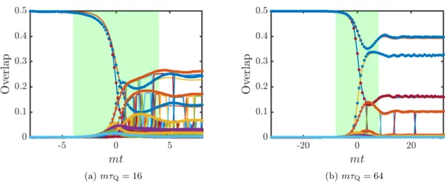
(a)mτQ= 16 (b)mτQ= 64

Figure 3.1: Overlaps of the evolving wave function with instantaneous eigenstates for two different ramps from the paramagnetic to the ferromagnetic phase with mτQ = 16 and mτ_Q= 64 for mL= 50 (m=M_i in terms of the initial mass). The green region indicates the non-adiabatic regime. Solid lines are TCSA data forN_cut= 25while dots are obtained from the numerical solution of the exact differential equations. Analytical results are plotted only for the few low-momentum states with the most substantial overlap. Lower indices in the legends refer to the quantum numbers of the modes present in the many-body eigenstate:pn=nπ/L. The composite structure of some lines is caused by level crossings experienced by multiparticle states.

Apart from this solution of the dynamics, we can calculate the population of energy eigenstates numerically with TCSA. This is a benchmark for our numerical method as it is contrasted with a numerically exact calculation. We can compare Eq. (3.6) with Eq.

(3.3) to express the overlapg of a state which consists of only a single particle pair with momentump:

| hp,−p|Ψ(t)i |²≡ |g_p(t)|² =n_p(t) Y

p⁰6=p

(1−n_p⁰(t)), (3.7) where the product goes over the infinite set of quantised momenta in finite volume. It is straightforward to generalise Eq. (3.7) to express the overlap of any state with the pair structure of the free spectrum with the time-evolved state.

In practice, we truncate this product at some finite pmax, since the goal is to match the analytic results with TCSA that operates with a truncation of its own. The one-mode cut-off of the analytic method and the many-body cut-off of TCSA cannot be brought to one-to-one correspondence with each other. However, overlaps are very sensitive to the number of states kept in each expansion, due to the constraint P

n|g_n|² = 1. Hence, our choice for the energy cutoff of TCSA for these figures is motivated by the goal to have the best possible match of the two approaches. Note that this is a single parameter for all the states.

The time evolution of the overlaps is presented in Fig. 3.1. Dots correspond to the solution of the differential equations for each mode and continuous lines denote TCSA data obtained by solving the many-body dynamics numerically. Fig. 3.1a depicts a curious behaviour of the second largest overlap in TCSA: the corresponding line seemingly consists of many different segments. This is a consequence of level crossings and the errors of numerical diagonalisation near these crossings. The state in question consists of two two- particle pairs and as the mass scaleM is ramped its energy increases steeper than that of high-momentum states with only a single pair, hence the level crossings. At each crossing

(17)

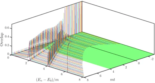
Figure 3.2: Instantaneous statistics of workP(W, t)along a ramp with mτ_Q= 16from the paramagnetic to the ferromagnetic phase formL= 50, obtained by TCSA withN_cut= 45.

The height corresponds to the time-dependent overlap squares. The green region indicates the non-adiabatic regime.

the numerical diagonalisation cannot resolve precisely levels in the degenerate subspace, so the resulting overlap is not accurate. This accounts for the most prominent difference between the numerical and analytical results. Apart from that, the agreement is quite satisfactory.

The light green background corresponds to the naive impulse regimet∈[−τ_KZ, τKZ].

Of course this is only a crude estimate for the time when adiabaticity breaks down as Eq.

(3.5) is strictly valid only as a scaling relation. Nevertheless, most of the change in each state population indeed happens within this coloured region. This statement is even more accentuated by Fig. 3.1b, that is, for a slower ramp. Comparing the two panels of Fig. 3.1 we observe that increasing the ramp time the probability of adiabaticity increases while the weight of the multiparticle states are suppressed. Note that although the two lowest available levels (the ground state and the first excited state) dominate the time-evolved state, the dynamics is far from being completely adiabatic that would mean no excitations at all. Hence, in accordance with the remarks concerning finite size effects in Sec. 2.1, we are within the regime of Kibble–Zurek scaling instead of being adiabatic.

We can also calculate the energy resolved version of the above figures, i.e. the instantaneous statistics of work, P(W, t). We present this quantity in Fig. 3.2. The different ridges correspond to “bands” of 2-particle, 4-particle etc. states with energy thresholds E= 2M,4M, . . .. The ridges diverge linearly in time, displaying the linear dependence of the gap on the linearly tuned M coupling. This figure illustrates the validity of the KZ arguments: low-energy bands dominate the excitations, and in each band, the modes with the lowest momenta (longest wavelengths) near the thresholds are the most prominent.

This feature is similar to what was observed on the lattice in Ref. [39].

3.1.2 The ferromagnetic-paramagnetic (FP) direction

The ferromagnetic ground state is twofold degenerate in infinite volume. For the initial state we choose the state with maximal magnetisation corresponding to the infinite volume

(18)

(a)mτQ= 16 (b)mτQ= 64

Figure 3.3: Overlaps of the evolving wave function with instantaneous eigenstates for two different ramps from the ferromagnetic to the paramagnetic phase with mτQ = 16 and mτ_Q= 64formL= 50(m=−M_iin terms of the initial mass). The green region indicates the non-adiabatic regime. Solid lines are TCSA data forN_cut= 31while dots are obtained from the numerical solution of the exact differential equations. Multiple pair states show several level crossings.

symmetry breaking state: |Ψ₀i = ^√¹₂(|0i_R+|0i_NS). As both sectors are present in the initial state, the time-evolved state also overlaps with both sectors. This provides yet another benchmark for our numerical approach and also a somewhat richer landscape of the overlap functions.

As one can see in Fig. 3.3, the dynamics are very similar to the PF case with the main difference coming from the fact that both sectors contribute. The different behaviour of the two vacua stems from the different available momentum modes in each sector: in the Ramond sector the momenta are larger in the lowest available modes and consequently they are less likely to be excited.

3.2 Ramps along the E₈ line

After investigating the free fermion line, we now turn to the behaviour of overlaps in the other integrable direction, i.e. for ramps along theE8 axis defined by the protocol

h(t) =−2h_it/τQ (3.8)

fort∈[−τ_Q/2, τ_Q/2].The scaling dimension of the perturbing operator σ is ∆_σ = 1/8, so critical exponentνis different in this direction from the free fermion case:ν = 1/(2−∆_σ) = 8/15 (cf. Eq. (2.14)). This implies that the Kibble–Zurek time (2.2) is given by

m1τKZ= (m1τQ)^8/23 , (3.9)

where, similarly to the free fermion case, the choice of the proportionality factor being 1 is just a convention.

Let us first take an overview of the dynamics by looking at the time-dependent work statisticsP(W, t) shown in Fig. 3.4.

Notice that in accordance with the Kibble–Zurek scenario, predominantly low-energy and low-particle modes get excited in the course of the ramp. In theE₈theory with multiple stable particles, the time evolved state has finite overlap not only with states consisting

(19)

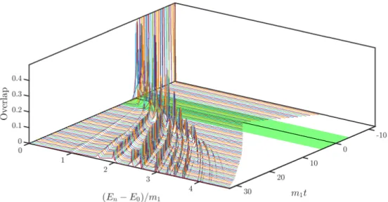
Figure 3.4: Instantaneous statistics of work P(W, t) for a ramp along the E8 axis with m₁τ_Q = 64, m₁L = 50, obtained by TCSA with N_cut = 45. The height corresponds to the time-dependent overlap squares. The green region indicates the non-adiabatic regime.

Notice the curvature of the “ridges” corresponding to the nonlinearm1∝h^8/15dependence of the mass gap on the distance from the critical point.

of pairs but also with states containing standing particles with zero momentum, including multiparticle states with a single such particle. We can observe that the energy distribution has peaks at some finite energy values, but low-momentum modes dominate for all branches (denoted by dashed lines of the same colour). This can be seen more clearly in Fig. 3.5 which presentsP(W) at the end of two ramps that differ in duration. Solid vertical lines indicate the energies of states consisting of standing particles only, i.e. combinations of particle masses.

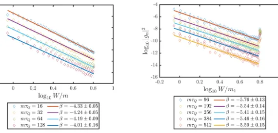
Let us remark that the perturbative calculations indicate that the KZ scaling applies to the overlap of each one-particle state and two-particle branch separately. That is a nontrivial statement since the spectrum of theE8 field theory is a result of a bootstrap procedure relying heavily on delicate details of the interaction, however, these details are overlooked by a first order perturbative calculation. Although we expect that the summed contribution of one- and two-particle states to the energy density satisfies the KZ scaling (in line with the generic reasoning of Sec. 2.1), the much stronger statement of APT concerning the scaling behaviour of separate branches does not necessarily hold true. This is in fact what we observe in Fig. 3.5: as the average excess heat diminishes, the overlap of low-lying states increase instead of decreasing. However, as we are going to show below, both quench times are within the KZ scaling region and the scaling of the excess heat does satisfy Eq. (2.6).

A remote analogy can be drawn with the form factor series expansion calculation of the central charge in integrable perturbed conformal field theories, where the result of the sum over multiparticle states is fixed by the c-theorem, while the separate terms vary greatly due to the details of the interaction [99]. We note that in the current case the ambiguity arises from taking the L → ∞ limit, since strictly speaking the adiabatic perturbation theory is sensible only if the ground state overlap remains close to1, which is impossible for a finite density state in the thermodynamic limit. Previous calculations within the APT framework illustrate that this condition can be relaxed when calculating intensive quantities [19, 40], demanding a low-density time-evolved state instead of one with almost unity

Kibble–Zurek mechanism in the Ising Field Theory K. Hódsági