Vortex confinement transitions in the modified Goldstone model

Vortex confinement transitions in the modified Goldstone model

Michikazu Kobayashi,^1,∗ Gergely Fej˝os,^{2, 3, 4,†} Chandrasekhar Chatterjee,^2,‡ and Muneto Nitta^{2, 5,§}

1Department of Physics, Kyoto University, Oiwake-cho, Kitashirakawa, Sakyo-ku, Kyoto 606-8502, Japan

2Research and Education Center for Natural Sciences, Keio University, Hiyoshi 4-1-1, Yokohama, Kanagawa 223-8521, Japan

3Department of Physics, Keio University, Hiyoshi 3-14-1, Yokohama, Kanagawa, 223-8522, Japan

4Institute of Physics, E¨otv¨os University, 1117 Budapest, Hungary

5Department of Physics, Keio University, Hiyoshi 4-1-1, Yokohama, Kanagawa 223-8521, Japan

The modified XY model is a variation of theXY model extended by a half periodic term, ex- hibiting a rich phase structure. As the Goldstone model, also known as the linear O(2) model, can be obtained as a continuum and regular model for theXY model, we define the modified Goldstone model as that of the modified XY model. We construct a vortex, a soliton (domain wall), and a molecule of two half-quantized vortices connected by a soliton as regular solutions of this model.

Then we investigate its phase structure in two Euclidean dimensions via the functional renormaliza- tion group formalism and full numerical simulations. We argue that the field dependence of the wave function renormalization factor plays a crucial role in the existence of the line of fixed points describ- ing the Berezinskii-Kosterlitz-Thouless (BKT) transition, which can ultimately terminate not only at one but at two end points in the modified model. This structure confirms that a two-step phase transition of the BKT and Ising types can occur in the system. We compare our renormalization group results with full numerical simulations, which also reveal that the phase transitions show a richer scenario than expected.

I. INTRODUCTION

The Berezinskii-Kosterlitz-Thouless (BKT) transition [1–4] is a topological phase transition of two-dimensional systems, which divides a low-temperature phase with bound vortex-antivortex pairs from a high temperature phase with free vortices. The phenomenon was first an- alyzed in terms of the XY model, and one of its most important impacts was that it showed that superfluidity and superconductivity can be realized even in two di- mensions. Even though in two dimensions long-range order with continuous symmetry is forbidden by the Coleman-Mermin-Wagner (CMW) theorem [5–7], there is a possibility of quasi-long-range order, which shows al- gebraically decaying correlations. The BKT transition realizes this scenario, and it also has the unique feature of being a continuous phase transition without break- ing any symmetry. It has been experimentally confirmed in various condensed matter systems such as ⁴He films [8], thin superconductors [9–13], Josephson-junction ar- rays [14, 15], colloidal crystals [16–19], and ultracold atomic Bose gases [20]. The XY model shares common properties including the BKT transition with the two- dimensional linear O(2), or Goldstone model at large dis- tances or low energies, which is a regular version of the XY model described by one complex scalar field, in which the U(1) Goldstone mode for the XY model is comple- mented by a massive amplitude (Higgs) mode. One of

∗michikaz@scphys.kyoto-u.ac.jp

†fejos@keio.jp

‡chandra.chttrj@gmail.com

§nitta@phys-h.keio.ac.jp

the merits of the latter is to allow vortices as regular so- lutions in contrast to the XY model in which vortices are singular configurations.

XY-like models do not necessarily show the BKT tran- sition. For example, for sharply increasing spin-spin po- tential, the phase transition between the paramagnetic and ferromagnetic phases can be of first order [21]. It is not surprising that the so-called modifiedXY model, where on a square lattice the Hamiltonian of the rotor is extended with aπperiodic term

H^mXY =−JX

hi,ji

cos(ϑi−ϑj)−J⁰X

hi,ji

cos[2(ϑi−ϑj)], (1) also shows a different scenario. It was predicted long ago that for large enoughJ⁰ coupling, there exists a nematic phase separated from the ferromagnet and the transition between them is of Ising type [22, 23]. This was also confirmed by numerical calculations [24]. The Ising-type transition is related to the presence of domain walls in this model. Moreover, it was conjectured that molecules and anti molecules of half-quantized vortices play a cru- cial role for phase transitions, in contrast to a pair of vortices and anti vortices in theXY model. As of today, the model (1) and its various modifications [25–33] are of great importance and interest, especially due to their relevance in condensed matter physics applications, e.g., superfluidity in atomic Bose gases [34], arrays of uncon- ventional Josephson junctions [35], or high-temperature superconductivity [36].

The BKT transition of the XY model was originally analyzed via a real-space renormalization group (RG) ap- proach [4], which is rather unconventional and not easily

2 linkable to the Wilsonian picture of the RG [37]. In the

past, the functional RG (FRG) approach, which adopts the Wilsonian idea of mode elimination and averaging to the level of the effective action [38], was also applied and developed in regard to the BKT transition in both continuum [39–43] and lattice formulations [44, 45]. It turned out that the conventional, Wetterich formulation of the method was capable of showing signs in the two- dimensional linear O(2) or Goldstone model of the line of fixed points that is responsible for the topological na- ture of the phase transition. This is remarkable in the sense that no vortices need to be introduced explicitly, as opposed to the older real-space RG description [4]. One of the shortcomings of the treatment, however, is that because one is typically solving the RG flow equation of the scale-dependent effective average action via a deriva- tive expansion, as an artifact, only a line of quasi-fixed points is found. That is, the RG flow does not stop along this line, but only slows down significantly compared to other regions of the parameter space. It is worth point- ing out that recently in a dual lattice formulation of the FRG, Krieg and Kopietz [45] exactly reproduced the RG flow equations derived by Kosterlitz and Thouless [4] and therefore the existence of a true line of fixed points was established in terms of a momentum space RG. It would be interesting, however, to develop a scheme in the ordi- nary Wetterich formulation of the FRG, which could also lead to a similar result.

The goal of this study is twofold. On the one hand, we aim to show a rather simple approximation scheme of the FRG flow equations that can show significant improve- ment on the possibility of reaching a true line of fixed points in the continuum version of the XY model, and more importantly argue that it can also be applied natu- rally to the modifiedXY model, i.e., the continuum ver- sion of (1). In the framework of a momentum space RG, we describe the two-step transition in the latter model and we will also predict that fluctuations may completely make the topological transition disappear. On the other hand, we also aim to provide full numerical simulation of the system and show that depending on the value of the self-coupling of the scalar field, the structure of the transitions is even richer than it is predicted by the RG.

The paper is organized as follows. In Sec. II we intro- duce the modified Goldstone model and construct clas- sical solutions, an integer vortex, a soliton, and a vortex molecule of two half-integer vortices connected by a soli- ton in that model. In Sec. III, after giving a brief review of the FRG, we reproduce some earlier results of the BKT transition via the FRG and also show the improvement announced above. Then this scheme is applied to the modified XY model and we show how a two-step tran- sition can emerge in the system. In Sec. IV we confirm this scenario via full numerical simulations and reveal the nature of the corresponding transitions. Section V is de- voted to a summary. In Appendix A we show how to derive the Hamiltonian of the modified Goldstone model from the microscopic lattice model of the modified XY

model, while in Appendix B we derive some of the cor- responding flow equations of the FRG.

II. MODEL AND SOLUTIONS A. Modified Goldstone model

In this study we are interested in the continuum ver- sion of the XY model, i.e., the Goldstone model and its modification [for its derivation from the microscopic Hamiltonian (1) see Appendix A]

H= Z

x

a|∇ψ|²+b|∇ψ²|²+λ

2 |ψ|²/2−ρ0

2 , (2) where ψ is a complex scalar field, and λ, a, and b are positive coupling constants. The continuum version of the standardXY model refers tob= 0 and in the modi- fiedXY model we haveb >0. The field equation can be obtained from the Hamiltonian (2) as

0 = δH

δψ^∗ =−a∆ψ−2b ψ^∗∆ψ²+λ 2

|ψ|² 2 −ρ0

ψ,(3)

which we call the modified Gross-Pitaevskii equation.

B. Classical solutions

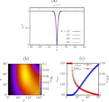
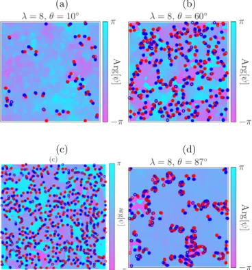
Field equations (3) of the modified Goldstone model admit superfluid (or global) vortex solutions. Here we show how such a vortex solution transforms into a half- quantized vortex molecule, when the second term of Eq. (2) becomes large enough. As we wish to compare our results with earlier works [24], in what follows we work in a simplified parameter space, wherea²+b²= 1, and thus thea= cosθandb= sinθparametrization can be used. As it turns out, this choice also helps perform the full numerical simulations of the thermodynamics of the system more easily. The transformation of the vor- tex solution can be seen in Fig. 1. One observes that around θ ≈ 78^◦, a clear picture of a vortex molecule emerges, where two half-quantized vortices are connected by a one-dimensional soliton. One expects that at finite temperature, as a function ofθ, somewhere close to the aforementioned value, the emergence of the molecules will have an effect on the phase structure of the system.

In a vortex molecule shown in Fig. 1, each of the two vortices has a half-quantized circulationR

d~l(∇~arg[ψ]) = πand the soliton connecting them has a π-phase jump.

To analyze the stability of the soliton, we determine the following one-dimensional stable solution of the modi- fied Gross-Pitaevskii equation (3) in one dimension with the boundary condition ψ(y → −∞) = √2ρ0, and ψ(y → ∞) = √2ρ0e^iϕ. Fig. 2 (a) shows the profiles of the soliton solutions, while Fig. 2 (b) shows the to- tal energy H^1D as a function of ϕ and θ. It is clear that if H^1D takes the maximum value at some ϕ < π,

FIG. 1. Vortex solution of the field equations transforms into a half-quantized vortex molecule around θ ≈ 78^◦ with the choiceρ0 = 1/2.

(a)

0 0.5 1

−30 −20 −10 0 10 20 30

|ψ|2

y ϕ=π

θ= 10^◦ 45^◦ 80^◦ 90^◦

(b)

0^◦ 60^◦ 120^◦ 180^◦ ϕ

0^◦ 30^◦ 60^◦ 90^◦

θ

0 0.02 0.04 0.06 0.08 0.1

H1D

(c)

90^◦ 120^◦ 150^◦ 180^◦

0◦ 30◦ 60◦ 90◦0 0.03 0.06 0.09

ϕmax ∆H1D

θ ϕmax

∆H_1D

FIG. 2. (a) Profiles of the amplitude |ψ|² of the soliton so- lutions for the modified Gross-Pitaevskii equation [Eq. (3)]

with θ = 10^◦ (black), θ = 45^◦ (red), θ = 80^◦ (blue), and θ = 90^◦ (green). (b) Dependence of the energy, H1D, on θ andϕ. (c) Dependence of the maximal angleϕmax and the energy barrier ∆H1Donθ. In the both panels, we setλ= 8 andρ0= 1/2.

then the soliton solution with ϕ = π becomes locally stable (metastable) by having a positive energy barrier

∆H^1D≡ H^1D(ϕ=ϕmax)− H^1D(ϕ=π), where the max- imal angle ϕ_max is the value of ϕ at which H^1D takes the maximum. Fig. 2 (c) shows the maximal angleϕ_max and the energy barrier ∆H^1D. The former starts to take a nonzero value, ∆H^1D >0, with ϕmax < π at around θ ≈ 15^◦, above which the soliton is, therefore, energet- ically stable. That is to say, the appearance of vortex molecules and the stability of the soliton are not related, and thus it is not the (de)stabilization of the domain wall that lets molecules emerge.

It is worth noting that these configurations become sin- gular in the limit ofλ→ ∞, in which the model reduces to the modifiedXY model. Therefore, the modifiedXY model doesnotallow these configurations as solutions to the field equations, while the modified Goldstone model does.

C. Type of symmetry and (quasi) breaking of symmetry

Here, we discuss the symmetry properties of the Hamil- tonian [Eq. (2)] and show the possible (quasi-)breaking patterns of symmetries. The symmetry of the Hamilto- nian with generic parameters is of U(1) as a phase shift of the field, ψ →ψe^iα for the arbitrary α∈ [0,2π). In the case ofa= 0 and b > 0, the two fields ψ andψ e^iπ

4 are identifiable, because the Hamiltonian [Eq. (2)] is the

functional ofψ²rather thanψ. Therefore, the symmetry of the Hamiltonian is only U(1)/Z2, where the Z2 sym- metry comes from the identification of ψ∼ ψ e^iπ. This Z²factor is essential for the presence of (deconfined) half- quantized vortices.

Depending on the parameter regions, the U(1) or U(1)/Z2symmetry is spontaneously broken in the ground state in different patterns summarized as follows:

U(1)^U(1)99K 1 fora >0 andb= 0, (4a) U(1)/Z2

U(1)/Z2

99K 1 fora= 0 andb >0, (4b) U(1)^U(1)/99K^Z2Z2 Z2

−→1 forba >0, (4c)

U(1)^U(1)=⇒1 fora≈b. (4d)

Here the arrows99K,−→, and =⇒denote quasi-breaking of symmetry via a BKT transition, ordinary symmetry breaking with a thermodynamic phase transition, and simultaneous (quasi)breaking of symmetry, respectively.

Here, quasibreaking means that the symmetry is not ex- actly broken due to the CMW theorem in the thermo- dynamic limit but is locally broken at semi macroscopic scales with an algebraically decaying correlation function.

Now let us explain each breaking pattern. In the sim- plest case, i.e., for a > 0 and b = 0 [Eq. (4a)], the standard BKT transition occurs with the quasibreaking of the U(1) symmetry. In the opposite case, i.e., fora= 0 andb >0 [Eq. (4b)], the BKT transition occurs with the quasi breaking of the U(1)/Z2 symmetry, for which half- quantized and anti-half-quantized vortices start to form in pairs. In the case of b a > 0 [Eq. (4c)], two suc- cessive spontaneous (quasi)breaking processes occur. At the first stage (at higher temperature) the U(1) symme- try is quasi broken to aZ2subgroup accompanied by the BKT transition. At the second stage, at a temperature lower than the BKT transition temperature, the remain- ingZ2symmetry is further spontaneously broken due to a thermodynamic transition. In this case, half-quantized and anti-half-quantized vortices start to form pairs at the BKT transition and domain walls appear at the thermo- dynamic transition. Some domain walls have no end- point forming loops as well as those in the Ising model, but some others appear between two half-quantized or two anti-half-quantized vortices forming vortex or anti- vortex molecules as shown in Fig. 1. In the remain- ing case of a≈b [Eq. (4d)], rather than a conventional BKT transition, the BKT transition occurs with the qua- sibreaking of U(1)/Z2symmetry and the thermodynamic transition with breaking ofZ²symmetry simultaneously.

All vortices are integers and domain walls do not have endpoints.

In the following sections, we study the modified Gold- stone model by the FRG and Monte Carlo simulation.

III. FUNCTIONAL RENORMALIZATION GROUP CALCULATIONS

In this section, after giving a brief review of FRG, we apply it to the modified Goldstone model approximately, at the leading order of the derivative expansion, and ob- tain the phase structure.

A. Flow equation: a review

Here we review the basics of the FRG. At the core of the formalism lies the Γk average effective action, in which fluctuations of the dynamical fields are incorpo- rated up to a momentum scalek. The Γ_k function obeys the flow equation:

∂_kΓ_k =1 2

Z

Tr [(Γ⁽²⁾_k +R_k)⁻¹∂_kR_k], (5) where Γ⁽²⁾_k is the second derivative matrix of Γk with respect to the dynamical variables andR_k is a regulator function, which is defined (in Fourier space) through a momentum-dependent mass term

1 2 Z

p,q

ψⁱ(q)R^ij_k(q, p)ψ^j(p), (6) added to the classical Hamiltonian (or Euclidean action).

We denoted the set of fluctuating field variables by ψ.

HereRk is supposed to give a large mass to modes that have momentaq.kand leave the ones with q&k un- touched. The classical Hamiltonian by definition does not contain any fluctuations; therefore, it serves as an initial condition for the RG flow of Γk=Λ at some mi- croscopic scale Λ. The flow equation (5) then needs to be integrated down tok= 0, where one obtains the full free energy (or quantum effective action). One is free to choose the Rk function such that it fulfills the require- ment of suppressing low-momentum modes, and in this paper we employ the so-called optimal version:

Rk(q, p) =Zk(2π)²(k²−q²)Θ(k²−q²)δ(q+p), (7) where Θ(x) is the Heaviside step function, andZ_k is the wave function renormalization factor.

B. Local potential approximation’

Here we solve flow equation (5) for the modified Gold- stone model approximately, using the ansatz for Γk,

Γk = Z

d²x Zk(ρ)

2 (∇ψⁱ)²+λk

2 (ρ−ρ0,k)²

, (8) where instead of a complex variable, theψⁱ field is con- sidered as a two-component real vector: ψⁱ = (ψ¹, ψ²), while ρ = ψⁱψⁱ/2, and we have only kept the original couplings in the effective potential. Namely, Eq. (8)

is compatible with the form of Eq. (2), but it comes with k-dependent couplings and a field-dependent wave function renormalization factor [Zk(ρ)]. In what fol- lows we will consider the Zk(ρ) function in two sepa- rate approximations: i)Zk(ρ)≈Zk(ρ0), andii)Zk(ρ)≈ Z_k(ρ₀) +Z_k⁰(ρ₀)(ρ−ρ₀). Approximation i) is sometimes called the local potential approximation’ (LPA’), with the prime referring to nontrivial wave function renormal- ization. First we work with the LPA’ and the next section is devoted to approximationii).

Projecting the flow equation (5) onto a subspace spanned by homogeneous field configurations, we get (see also Appendix B)

k∂k¯λk=−2¯λk[1−η_k⁽⁰⁾] + λ¯²_k

2π 1−η⁽⁰⁾_k 4

!

×

1 + 9

(1 + 2 ¯ρ0,kλ¯k)³

,(9a)

k∂_kρ¯_0,k=−η⁽⁰⁾_k ρ¯_0,k+ 1

4π 1−η⁽⁰⁾_k 4

!

×

1 + 3

(1 + 2 ¯ρ_0,kλ¯_k)²

,(9b)

where we have introduced dimensionless rescaled vari- ables ¯λk =λkk⁻²Z_k⁻² and ¯ρ0,k = ρ0,kZk. Here, η⁽⁰⁾_k =

−k∂kZk/Zk is the anomalous dimension at this order of the approximation, where the wave function renormal- ization is evaluated at the minimum point of the effec- tive potential, Z_k ≡Z_k( ¯ρ_0,k) (from now on we think of the wave function renormalization as a function of the rescaled field). If we project Eq. (5) onto ∼ (∇ψ^t)², where the index refers to the transverse direction, we ar- rive at the flow equation forZ_k (see, again, Appendix B for details),

k∂kZk( ¯ρ) =−Zk( ¯ρ) ρ¯λ¯²_k/π

(1 + ¯M_l,k² )²(1 + ¯M_t,k² )², (10) where ¯M_l,k² = M_l,k² /Zkk² and ¯M_t,k² =M_t,k² /Zkk², while M_l,k² and M_t,k² are the longitudinal and transverse com- ponents of the momentum independent part of the Γ⁽²⁾_k matrix, respectively,

M_l,k² =λk(3ρ−ρ0,k), M_t,k² =λk(ρ−ρ0,k), (11) and thus

M¯_l,k² = ¯λk(3 ¯ρ−ρ¯0,k), M¯_t,k² = ¯λk( ¯ρ−ρ¯0,k). (12) Since in Eqs. (9) it isZk =Zk( ¯ρ0,k) that appears through η⁽⁰⁾_k , we evaluate Eq. (10) at ¯ρ= ¯ρ_0,k and get

η_k⁽⁰⁾= ρ¯0,kλ¯²_k

π(1 + 2 ¯ρ0,kλ¯k)². (13) Now we can search for fixed points of Eqs. (9) and (13).

The flow diagram in terms of ¯λ_kand ¯ρ_0,kcan be seen on the left side of Fig. 3. We observe the line of quasifixed points and notes that the flow, even though significantly slowed down, is clearly nonzero in the aforementioned region.

C. Wave function renormalization improvement The key to the improvement to be described here is to realize how crucial the role of the wave function renor- malization factor Zk is in the previous description. In order to escape from the CMW theorem, in the low- temperature phase Z_k has to diverge so that the renor- malized field can condense (the expectation value of the bare field is always zero). Since any rescaling of the field should lead to the same description of the system, one ex- pects that any field derivative of the wave function renor- malization factor is proportional toZk itself,Z_k⁽ⁿ⁾∼Zk, which means that they also diverge, and in principle none of them should be neglected, as also pointed out, e.g., in [41]. As announced in the preceding section, here we take into account the first derivative ofZk, which will in- deed lead to a significant improvement in stabilizing the flow along the (quasi)line of fixed points, but more im- portantly, it also makes it possible to treat the modified Goldstone model in the FRG.

If we keep track of the field derivative ofZ_k, then it is possible to take into account in ηk the implicit k de- pendence coming from the change of the minimum of the effective potential when the RG scale is varied, similarly to what was done in earlier works, e.g., [46, 47]. In prin- ciple, we should have

ηk =−kdkZk

Z_k =−k∂kZk+Z_k⁰k∂kρ¯0,k

Z_k

=η_k⁽⁰⁾−wkk∂kρ¯0,k≡η⁽⁰⁾_k + ∆ηk, (14) whered_k refers to total differentiation and on the right- hand side bothZ_k andZ_k⁰ are evaluated at ¯ρ= ¯ρ_0,k. We have also introduced the notation ∆ηk = −wkk∂kρ¯0,k

withwk =Z_k⁰/Zk. SinceZ_k⁰ has appeared in our formula, we also need to derive a flow equation for it. This can be obtained from Eq. (10) after applyingd/dρ¯to the both sides (note that∂_k does not commute withd/dρ). Using¯ thatdM¯_l,k² /dρ¯= 3¯λ_k anddM¯_t,k² /dρ¯= ¯λ_k, we get

k∂_kZ_k⁰( ¯ρ_0,k)/Z_k( ¯ρ_0,k) = (15) 4 ¯ρ²_0,k¯λ²_k+ 6 ¯ρ0,kλ¯k+ 2 ¯ρ0,kwk−1

π(1 + 2¯λkρ¯0,k)³ +wkη⁽⁰⁾_k , which leads to

k∂kwk= 4 ¯ρ²_0,kλ¯²_k+ 6 ¯ρ0,kλ¯k+ 2 ¯ρ0,kwk−1 π(1 + 2¯λkρ¯0,k)³

+ 2w_kη_k⁽⁰⁾−w²_kk∂_kρ¯_0,k. (16) At this point, it is important to mention that Eq. (15)

6

-5 0 5 10 15 20 25 30 10ρ_0,k

5 10 15 20λ_k

(a)

-5 0 5 10 15 20 25 30 10ρ_0,k

5 10 15 20λ_k

(b)

FIG. 3. Comparison of (a) the leading order flow diagram with (b) the wave function renormalization improved one. The red flows are stopped at (a)t=−log(k/Λ) = 10 and (b)t= 200 (b), which shows that a significant stabilization of the line of fixed points is achieved with the improved approximation. For completeness, the blue flows are stopped at (a)t= 1,5,5,8 and (b)t= 2,8.5,20,40 (b), respectively.

is not exact, as deriving Eq. (10) we let the field op- erators act only on the potential part of the two-point correlation function and not onZk(ρ). This would have introduced a furtherZ_k⁰(ρ) dependence on the right-hand side of Eq. (10), which is neglected here. The reason be- hind this is that we think of the scheme in question as a first correction to the LPA’ in the sense that we are mo- tivated to derive the flow ofwk in the background flows of Zk, ¯λk, and ¯ρ0,k of the LPA’, which by definition are not affected explicitly by wk itself.

Now, once we return to the aforementioned flows, i.e., Eqs. (9), we notice that they do depend implicitly onw_k, but only because of the new expression of the anomalous dimensionη⁽⁰⁾_k →ηk =η_k⁽⁰⁾+ ∆ηk. This does not make much of a difference in the flow of ¯λk, but changes that of ¯ρ0,k. The reason is that Eq. (9b) becomes an implicit equation, since k∂_kρ¯_0,k also appears on the right-hand side through ∆η_k ≡ −w_kk∂_kρ¯_0,k. After some algebra we arrive at

k∂kρ¯0,k=

−η⁽⁰⁾_k ρ¯0,k+_4π¹

1−^η

(0) k

4

h

1 +_{(1+2 ¯ρ}³

0,kλ¯k)²

i

1−w_kh

¯

ρ_0,k+_16π¹

1 + _{(1+2 ¯ρ}³

0,k¯λ_k)²

i .

(17) The flow of ¯λk is analogous to Eq. (9a), but η⁽⁰⁾_k is re- placed byη_k:

k∂k¯λk =−2¯λk[1−ηk] + λ¯²_k 2π

1−ηk

4

×

1 + 9

(1 + 2 ¯ρ0,kλ¯k)³

.(18) Now we solve the coupled equations (13), (16), (17) and (18). The corresponding flow diagram can be seen on the right-hand side of Fig. 3. The comparison shows that taking into account the derivative of the wave function renormalization factor in the anomalous dimension sig- nificantly stabilizes the flow along the line of (quasi-)fixed

points, as in the improved case the freezing of the flow holds on∼20 times longer in RG timet=−log(k/Λ).

D. Phase structure

Now we are in a position to show that in the modi- fiedXY model fluctuations can dramatically change the structure of the line of fixed points, as seen in Fig. 3.

First, note that, the ansatz of Eq. (8) and the approxima- tionZ_k( ¯ρ)≈Z_k( ¯ρ_0,k) +Z_k⁰( ¯ρ_0,k)( ¯ρ−ρ¯_0,k) is compatible with the microscopic Hamiltonian of the modified XY model, since from Eq. (8) we have

Γk= Z

d²xhZk+Z_k²wk(ρ−ρ0,k) 2 (∇ψⁱ)² +λ_k

2 (ρ−ρ_0,k)²i

, (19)

which is equivalent to Γk=

Z d²x

ak(∇ψⁱ)²+ 4bk(ψ^j)²(∇ψⁱ)² +λ_k

2 (ρ−ρ_0,k)²

, (20)

wherea_k = (Z_k−Z_k²w_kρ_0,k)/2 andb_k =Z_k²w_k/16. Eq.

(20) is now of the form of the original Hamiltonian in Eq. (2) using theψⁱ vector notation.

The reason why the RG flows of the ordinary XY model can change dramatically is that depending on the initial valuewΛ(orbΛ, equivalently) at the UV scale, ¯ρ0,k

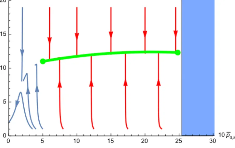
can approach a singularity, which sends the flows in the

¯λk- ¯ρk plane away from the line of fixed points. What es- sentially happens is that the line of quasifixed points ter- minates also at another end point (Fig. 4). The end point on the left corresponds to a BKT transition at higher temperature and the new one on the right signals an- other transition at lower temperature. Even though the method does not make a definite prediction, this should

FIG. 4. Flow diagram for the modifiedXY model with the initial conditionwΛ= 0.4. The red curves end on the line of fixed points, while the blue ones deviate from it. The fixed line is terminating at two endpoints, the left one corresponding to the high-temperature transition (BKT) and the right one controlling the low-temperature transition. The position of the latter depends on the initial valuewΛ (note that the position of the former is not sensitive towΛ, if it exists). The flows become divergent in the shaded region of the parameter space in accordance with (21).

correspond to the Ising transition already reported in ear- lier papers [22–24].

Analyzing the flow of ¯ρk, we note that already in the ordinary XY model, i.e., for wΛ = 0, at first sight it might seem possible that the denominator on the right- hand side of Eq. (17) becomes zero, but it turns out that this never happens. The flow equation always makeswk

decrease as fluctuations are integrated out, and therefore the flows are regular. Note, however, if at the microscopic scale,wΛ>0, thenk∂kρ¯0,kcan indeed blow up.

The condition that needs to be met for a diverging flow is

w_Λ⁻¹<ρ¯0,Λ+ 1 16π

1 + 3

(1 + 2 ¯ρ_0,Λλ¯_Λ)²

, (21) which shows that for positive wΛ values the line of fixed points can also terminate on the right (see Fig. 4), leading to a two-step transition. For later reference, just as in Sec. II, we restrict ourselves to the case

a²_Λ+b²_Λ= 1, (22) i.e., we may use the parametrization a_Λ = cosθ and bΛ = sinθ (θ ∈ [0, π/2]), which leads to the following constraints:

cosθ=ZΛ(1−ZΛwΛρ0,Λ)/2, (23) sinθ=Z_Λ²wΛ/16. (24) Solving them forw_Λ andZ_Λ, we get

Z_Λ= 2(cosθ+ 8ρ_0,Λsinθ), (25) wΛ= 4 sinθ

(cosθ+ 8ρ_0,Λsinθ)². (26) Dropping the last term in the large parantheses of the right-hand side of Eq. (21) (we are interested in a rough

estimate), we can get the following condition for the crit- ical value ofρ0,Λbelonging to the second endpoint of the line of (quasi)fixed points:

0 =−(cosθ+ 8ρ0,Λsinθ)² 4 sinθ

+ 2(cosθ+ 8ρ_0,Λsinθ)ρ_0,Λ+ 1

16π. (27) For a given θ, we solve this equation for ρ0,Λ (see the endpoint on the right-side of Fig. 4). Surprisingly, ifθ6= 0 is small, i.e. we are close to theXY model, the solution ρ0,Λ|^sol is always negative. This means that since the flows blow up for initial values ρ0,Λ > ρ0,Λ|^sol, unless

¯

ρ0,Λ|^sol ≡ZΛρ0,Λ|^sol ≈0.5 (which is the location of the original endpoint of the BKT transition), the line of fixed points completely disappears. The critical angle at which this happens is

θc ≈86.8^◦. (28) That is to say, for 06=θ < θc, if there is a transition in the system, it cannot be of topological type, no matter how close we are to theXY model (still, atθ= 0 we have one, and only one BKT transition). However, onceθ > θ_c, the line of fixed points starts to return to the picture, now equipped with another end point, which indicates that there exist two transitions. A higher-temperature transi- tion has to be of BKT type and a lower-temperature tran- sition, presumably an Ising transition [24], is expected to be of second order. Note that the aforementioned struc- ture heavily relies on the assumptiona²_Λ+b²_Λ= 1. Had we not had this constraint and just set, e.g.,aΛ≡1, we would have found a two-step transition for 0 < b < bc

(the higher-temperature one being topological), and no topological transition for b > b_c (here b_c > 0 is some positive constant).

8 IV. NUMERICAL SIMULATIONS

In this section we numerically investigate the equilib- rium properties of the modified Goldstone model defined in Eq. (2).

A. Preparation

The discretized Hamiltonian H^∆x from Eq. (2) be- comes

H^∆x=H¹+H², H¹=aX

hi,ji

|ψ_i−ψ_j|²+bX

hi,ji

|ψ²_i −ψ_j²|², H²=λ∆x²

2 X

i

(|ψ_i|²/2−ρ₀)²,

(29)

where ψi is the field ψ at the discretized point ~x= ~xi

and ∆xis the lattice spacing (which serves as an ultra- violet cutoff scale). In the limit ofλ→ ∞and rewriting ψ=√2ρ0e^iθi, the discretized HamiltonianH^∆xbecomes equivalent to the Hamiltonian H^mXY in Eq. (1) for the modifiedXY model withJ = 4aρ₀ andJ⁰ = 8bρ²₀.

Now we numerically calculate equilibrium ensemble av- erages

hfi=

Z Y

i

dψidψ^∗_i

! X

i

f e^−H∆x/T

Z Y

i

dψidψ_i^∗

! X

i

e^−H∆x/T

, (30)

by using the Monte Carlo technique. First, by fixing the amplitude |ψ_i|of the field, we use the cluster Monte Carlo technique with the Wolff algorithm [48]. Then, to accelerate the equilibration process, we alternately apply the Wolff algorithm to equilibrate the phaseθi= arg[ψi] and the standard Metropolis-Hastings algorithm to equi- librate the amplitude|ψ_i|. For numerical parameters, we have used ∆x= 1,ρ₀= 1/2. Similarly to the preceding section, we parametrize aandb as in Eq. (22),

a= cosθ, b= sinθ, a²+b²= 1. (31)

B. Correlation function and transition temperature We first show our results for the two correlation func- tions

G₁(r) =X

i

X

r≤|xj|<r+∆x

∆x²hψ_i+j^∗ ψii N(r)L² , G2(r) =X

i

X

r≤|xj|<r+∆x

∆x²hψ_i+j^∗2ψ_i²i N(r)L² ,

(32)

where L is the system size and N(r) is the number of points, xi, that satisfy r ≤ |xi| < r + ∆x. When θ = 0 (θ = π/2), we expect the standard BKT tran- sition triggered by integer vortices (half-quantized vor- tices) for ψi (ψ²_i) and the algebraic decay G1(r)∝ r^−η [G₂(r) ∝ r^−η] below the BKT transition temperature.

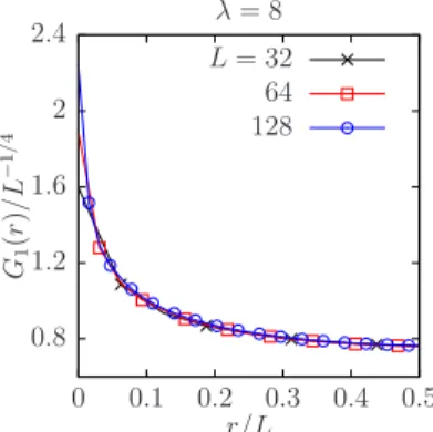
At the BKT transition temperature, the critical expo- nent satisfies η = 1/4 [3, 4]. To obtain the BKT tran- sition temperature, therefore, we can use the finite-size scaling of the correlation functions, in whichG^(1,2)/r^−1/4 is expected to be a universal function ofr/L. Figure 5

0.8 1.2 1.6 2 2.4

0 0.1 0.2 0.3 0.4 0.5 G1(r)/L−1/4

r/L λ= 8 L= 32

64 128

FIG. 5. Finite-size scaling ofG1(r) withθ = 0 and λ = 8 at the BKT transition temperatureT₁^BKT= 0.60T^∗ with the critical exponent η = 1/4. The system sizes are L = 32 (crosses),L= 64 (open squares), andL= 128 (open circles).

We use the same symbols for the system sizeL in all other figures unless otherwise noted.

shows the dependence of G1(r)/L^−1/4 with θ = 0 and λ = 8 as a function of r/L at T = 0.6T^∗ where T^∗ is the BKT transition temperature for the standard XY model with θ = 0 and λ → ∞. The expected univer- sality ofG₁(r) is sufficiently satisfied at large r, which, therefore, predicts that the BKT transition temperature isT₁^BKT'0.6T^∗. In the same way, we can estimate the temperature T₂^BKT ' 0.21T^∗ with θ = π/2 and λ = 8 from the finite-size scaling ofG2(r).

We further expect the appearance of a second-order, Ising-type phase transition [24], where the domain of def- inition for the phase of theψfield is spontaneously bro- ken from [0,2π] to [0,π], which can be thought of as a spontaneous breaking of a discreteZ2 symmetry. At the critical temperature for this phase transition, the cor- relation function also shows algebraic decay. Since the critical exponent η takes the same value as that of the BKT transition temperature, i.e., η = 1/4 for the two- dimensional Ising-type transition, we can use the same finite-size scaling analysis as shown in Fig. 5. We here define the temperature T₁ (T₂) at which G₁(r) [G₂(r)]

shows the algebraic decay G₁ ∝r^−1/4 [G₂(r)∝ r^−1/4].

Then, by definition,T1=T₁^BKT atθ= 0 andT2=T₂^BKT at θ = π/2. Denoting by θ1 and θ2 critical angles, we have found the following results forT1 andT2.

1. Whenθis small, i.e.,θ≤θ1, thenT1> T2.

2. Whenθ is large, i.e.,θ₂< θ < π/2, thenT₁< T₂. 3. When λ is finite, then θ1 < θ2. For θ1 < θ ≤θ2,

neitherG₁(r) norG₂(r) satisfiesG_1,2(r)∝r^−1/4at any temperatures and bothT1 andT2 are absent.

4. When λ → ∞ for the modified XY model, then θ₁=θ₂, i.e., bothT₁ andT₂ always exist at anyθ.

λ θ1 θ2

8 50.8^◦ 84.5^◦ 16 66.0^◦ 79.6^◦

∞ 64.2^◦

TABLE I. Specific values ofθ1 and θ2 at λ= 8, 16, and∞ (modifiedXY model).

The specific values ofθ1 andθ2 are shown in Table I.

C. Superfluid density and specific heat To determine the type of the transitions, we calculate the superfluid densityρ_sdefined as [49, 50]

ρs= 1

(a+ 4b)L² lim

δ→0

F(δ)−F(0)

δ² (33)

and the specific heat C = dhHi/dT, where F(δ) =

−Tloghe^−H/Ti is the free energy under the argument- twisted boundary conditionψ(x+L) =e^iδ·Lψ(x). When a BKT transition occurs at the transition temperature T^BKT, the universal jump ∆ρ_s of the superfluid density is

∆ρs= T^BKT

π . (34)

On the other hand, for second-order transitions we expect close to the corresponding critical temperature (T^2nd) that the superfluid density obeysρs∝(T^2nd−T)^ζ. The critical exponentζis obtained by the Josephson relation ζ= 2β−νη, whereβ,ν, andη are the critical exponents of the order parameter, the correlation length, and the correlation function, respectively. By insertingβ = 1/8, ν = 1, and η = 1/4 for the Ising-type transition, we obtainζ= 0, i.e., the superfluid density also jumps at the transition temperature, similarly to the BKT transition.

However, no universal relation holds, which allows for a distinction between the two.

Figure 6 shows the dependence of the superfluid den- sity with respect to the temperature forθ= 0^◦[Fig. 6(a)]

and θ = 10^◦ [Fig. 6(b)]. The solid line shows the rela- tion ρs =T /π. In Fig. 6(a) this line intersects ρs with a good accuracy at T1, suggesting the standard univer- sal relation related to the BKT transition temperature, i.e., we indeed observe a topological transition. In Fig.

6(b), however, ρ_s deviates from the aforementioned line at T1 and therefore we expect that the transition is of

(a)

0 0.2 0.4 0.6 0.8 1

0 0.2 0.4 0.6 0.8 ρs/ρ

T /T^∗ λ= 8,θ= 0^◦

(b)

0 0.2 0.4 0.6 0.8 1

0 0.2 0.4 0.6

ρs/ρ

T /T^∗ λ= 8,θ= 10^◦

FIG. 6. Temperature dependence of the superfluid density ρs for λ= 8 at (a)θ = 0^◦ and (b) θ = 10^◦ [the panel (b)].

The solid, dashed, and dash-dotted lines show the relation ρs=T /π, whereT =T1, andT =T2, respectively.

second order, with a nonuniversal jump at the transition temperature. Here we relabel T1 ≡T₁^2nd. In neither of the panels do we find any characteristic structure inρ_sat T =T₂. We therefore conclude that the property of the correlation functionG2∝r^−1/4 is just the crossover and we relabelT2 as the crossover temperatureT2≡T₂^CO.

(a)

0 0.2 0.4 0.6 0.8 1

0 0.1 0.2 0.3

ρs/ρ

T /T^∗ λ= 8,θ= 60^◦

(b)

0 0.2 0.4 0.6 0.8 1

0 0.1 0.2 0.3

ρs/ρ

T /T^∗ λ= 8,θ= 87^◦

FIG. 7. Temperature dependence of the superfluid densityρs

forλ= 8 and (a) θ = 60^◦ and (b)θ = 87^◦. The solid line shows the relation ρs = T /π. The dash-double-dotted line in (a) shows the estimated first-order transition temperature T∗^1st. The dashed and the dash-dotted lines (b) showT=T1

andT=T2, respectively.

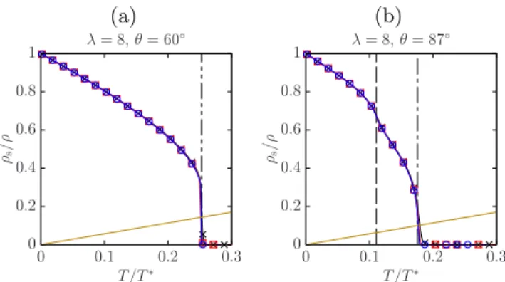
Figure 7 shows the dependence of the superfluid den- sity on the temperature for θ = 60^◦ [Fig. 7(a)] and θ = 85^◦ [Fig. 7(b)]. As shown in Table I, the value θ= 60^◦ is betweenθ1 andθ2 forλ= 8, and we find nei- ther a BKT nor a second-order phase transition. Instead, what we see is a first order phase transition due to the sharp jump of the superfluid densityρs [see Fig. 7 (a)].

Because the temperature at which the superfluid density ρs jumps does not really depend on the system size L, its estimation is fairly simple. We denote this transition temperature byT_∗^1st. In Fig. 7 (b), i.e., forθ= 87^◦,θis larger thanθ2and the superfluid densityρsdoes show the universal relation (34) at the corresponding temperature, T =T₂. Therefore, we find again a BKT transition with the aforementioned transition temperature, relabeling it

10 as T₂≡T₂^BKT.

(a)

0 1 2 3 4 5

0^◦ 30^◦ 60^◦ 90^◦

∆ρs/∆ρs0

θ λ= 8

(b)

0 1 2

0^◦ 30^◦ 60^◦ 90^◦

∆ρs/∆ρs0

θ λ= 16

FIG. 8. Jump of the superfluid density ∆ρs normalized by

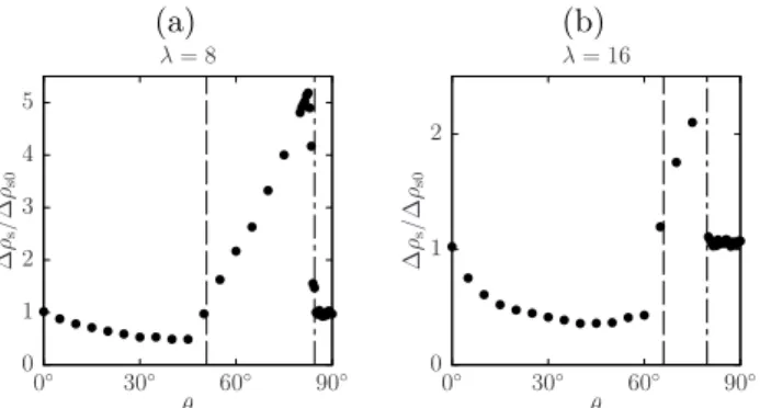
∆ρs0 for (a)λ = 8 and (b) λ= 16. The dashed and dash- doted lines showθ1 andθ2, respectively.

Figure 8 shows the jump of the superfluid density ∆ρ_s at the phase transition as a function ofθ, normalized by

∆ρs0, which is the value for the universal jump (34) for the BKT transition. It is specifically defined as (note that T₁,T_∗^1st, andT₂ depend onθ)

∆ρ_s0=













 T1

π, 0≤θ < θ1

T_∗^1st

π , θ1≤θ < θ2

T₂

π, θ2≤θ≤π 2.

(35)

We estimate the value of the jump ∆ρs by fitting the superfluid density ρs at the transition temperature, i.e.

T1 for 0 ≤ θ < θ1, T_∗^1st for θ1 ≤ θ < θ2, and T2 for θ₂≤θ≤π/2, via the function

ρs(θ, L) = ∆ρs(θ) +a(θ)

L , (36)

whereais aθ-dependent constant. Forθ= 0 andθ > θ2, the relation ∆ρs ' ∆ρs0 is satisfied; therefore, we find BKT transitions with the transition temperature T₁^BKT forθ= 0 and T₂^BKT for θ₁≤θ≤π/2. For other values, the universal relation does not hold and the transition becomes of second order for 0 < θ < θ1, and of first order forθ1< θ≤θ2.

Figure 9 shows the specific heatC. Whereas the spe- cific heat has a single peak near the transition tempera- ture forθ < θ2, i.e., in Figs. 9(a)-(c), it has double peaks forθ≥θ2, suggesting two-step transitions. In the latter case, the first and second peaks of the specific heat cor- respond to the temperaturesT₁andT₂, respectively. Be- cause the correlation functionG1becomesG1∝r^−1/4at T =T1 and the phase atT < T1 should be continuously connected from the phase withθ < θ2 (see Fig. 10), the transition at T1 should indeed be of second order. The absence of the peak at T = T₂ for θ < θ₁ consolidates our conclusion that hereT₂gives not the transition, but only a crossover as T₂^CO.

(a)

1 1.2 1.4 1.6

0 0.2 0.4 0.6 0.8

C

T /T^∗ λ= 8,θ= 0^◦

(b)

0.8 1.2 1.6 2 2.4

0 0.2 0.4 0.6

C

T /T^∗ λ= 8,θ= 10^◦

(c)

XJ10339WPRRESEARCHDecember 30, 201917:52

Important Notice to Authors

No further publication processing will occur until we receive your response to this proof.

Attached is a PDF proof of your forthcoming article in Physical Review Research. Your article has 14 pages and the Accession Code isXJ10339W.

Please note that as part of the production process, APS converts all articles, regardless of their original source, into standardized XML that in turn is used to create the PDF and online versions of the article as well as to populate third-party systems such as Portico, Crossref, and Web of Science. We share our authors’ high expectations for the fidelity of the conversion into XML and for the accuracy and appearance of the final, formatted PDF. This process works exceptionally well for the vast majority of articles; however, please check carefully all key elements of your PDF proof, particularly any equations or tables.

Figures submitted electronically as separate files containing color appear in color in the journal.

Specific Questions and Comments to Address for This Paper 1Please seehttp://publish.aps.org/authors/new-novel-policy-physical-reviewfor information regarding claims of priority

and check modification.

2 Please note that Phys. Rev. style discourages the use of one-sentence paragraphs.

3Please seehttp://publish.aps.org/authors/logarithms-h14for information regarding logarithms and specify the base of the logarithmic function, if needed, throughout.

4 Please check substitution of “O” for “O” to denote order of.

Q: This reference could not be uniquely identified due to incomplete information or improper format. Please check all information and amend if applicable.

ORCIDs: Please follow any ORCID links ( ) after the author names and verify that they point to the appropriate record for each author.

Open Funder Registry: Information about an article’s funding sources is now submitted to Crossref to help you comply with current or future funding agency mandates. Crossref’s Open Funder Registry (https://www.crossref.org/services/funder-registry/) is the definitive registry of funding agencies. Please ensure that your acknowledgments include all sources of funding for your article following any requirements of your funding sources. Where possible, please include grant and award ids. Please carefully check the following funder information we have already extracted from your article and ensure its accuracy and completeness:

MEXT, S1511006 JSPS, 16H03984, 19K14713, 18H01217 National Research, Development and Innovation Office, 127982 Hungarian Academy of Sciences KAKENHI, 15H05855 MEXT Other Items to Check

• Please note that the original manuscript has been converted to XML prior to the creation of the PDF proof, as described above.

Please carefully check all key elements of the paper, particularly the equations and tabular data.

• Title: Please check; be mindful that the title may have been changed during the peer-review process.

• Author list: Please make sure all authors are presented, in the appropriate order, and that all names are spelled correctly.

• Please make sure you have inserted a byline footnote containing the email address for the corresponding author, if desired.

Please note that this is not inserted automatically by this journal.

• Affiliations: Please check to be sure the institution names are spelled correctly and attributed to the appropriate author(s).

• Receipt date: Please confirm accuracy.

• Acknowledgments: Please be sure to appropriately acknowledge all funding sources.

• Hyphenation: Please note hyphens may have been inserted in word pairs that function as adjectives when they occur before a noun, as in “x-ray diffraction,” “4-mm-long gas cell,” and “R-matrix theory.” However, hyphens are deleted from word pairs when they are not used as adjectives before nouns, as in “emission by x rays,” “was 4 mm in length,” and “theRmatrix is tested.”

Note also that Physical Review follows U.S. English guidelines in that hyphens are not used after prefixes or before suffixes:

superresolution, quasiequilibrium, nanoprecipitates, resonancelike, clockwise.

• Please check that your figures are accurate and sized properly. Make sure all labeling is sufficiently legible. Figure quality in this proof is representative of the quality to be used in the online journal. To achieve manageable file size for online delivery, some compression and downsampling of figures may have occurred. Fine details may have become somewhat fuzzy, especially

(d)

0 5 10 15 20 25

0 0.1 0.2 0.3

C

T /T^∗ λ= 8,θ= 87^◦

FIG. 9. Temperature dependence of the specific heatC for λ= 8 and (a)θ = 0^◦, (b)θ = 10^◦, (c)θ= 60^◦, and (d)θ = 87^◦. The dash-double-dotted line in (c) shows the estimated first-order transition temperatureT∗^1st. The dashed and dash- dotted lines in (a), (b), and (d) showT =T1 and T =T2, respectively.

D. Phase diagram

Figure 10 shows the phase diagram of the modified Goldstone model in Eq. (29). For θ = 0, there is the standard BKT transition with the transition tempera- tureT1≡T₁^BKT. AtT < T₁^BKT, integer vortex pairs are bounded to show a quasi-long-range ordered phase. For 0 < θ < θ₁, this BKT transition changes to a second- order phase transition with the transition temperature T1 ≡ T₁^2nd, implying a true long-range-order phase for T < T₁^2nd with the breaking of the Z2 symmetry. For θ1 ≤ θ < θ2, the two temperatures T₁^2nd and T₂^CO de- fined for 0< θ < θ₁ merge to one first-order transition temperature,T_∗^1st. Forθ₂≤θ≤π/2, this transition tem- perature, T_∗^1st, splits again into two transition tempera- tures T₁^2nd and T₂^BKT. The second-order phase transi- tion ultimately disappears, as whileθ→π/2,T₁^2nd →0.

Unlike the BKT transition for θ = 0, the BKT transi- tion for θ₂ ≤ θ ≤ π/2 is triggered by the correlation functionG2(notG1), and therefore we expect the quasi- long-range order phase by the bounding of half-quantized vortex pairs at T₁^2nd < T < T₂^BKT. Because the low- temperature phases, i.e., T < T_∗^1st forθ1 ≤θ < θ2 and T < T₁^2nd forθ₂≤θ≤π/2, should be continuously con- nected to the long-range-order phase at 0< θ < θ₁, these phases should also be of true long-range order.